Representation Learning for Spatiotemporal Physical Systems

Paper: arXiv:2603.13227 Code: helenqu/physical-representation-learning Code reference: main @ bb77f7b5 (2026-03-18)

1. Motivation (研究动机)

这篇论文关心的不是“能否把物理仿真的下一帧画准”，而是“模型学到的表征是否真的保留了支配系统演化的物理信息”。在 PDE-governed spatiotemporal systems 中，常见路线是训练一个 autoregressive surrogate model：给定若干历史场，逐步预测后续 full-field state，用神经网络替代昂贵的数值求解器。这个目标在工程上很自然，但作者指出它有两个结构性瓶颈：第一，逐像素或逐网格点预测要求模型复原大量低层细节，训练开销高；第二，autoregressive rollout 会把单步误差不断累积，最后的可视化质量或短期预测误差未必能说明模型理解了系统的 governing parameters。

论文提出的评估视角更偏科学任务：如果一个表示 $z = f (x)$ 真正捕获了物理过程，那么从它上面应该能恢复系统参数，例如 active matter 中的 active dipole strength $α$ 与 alignment strength $ζ$ ，shear flow 中的 Reynolds number 与 Schmidt number，Rayleigh-Bénard convection 中的 Rayleigh number 与 Prandtl number。参数估计比“下一帧像不像”更接近科学解释，因为这些参数决定轨迹的相变、涡旋、对流单元、湍流倾向和长期演化形态。用 frozen encoder + probe 的方式做参数回归，也能把“预训练表征中已经有多少物理信息”与“下游监督头学习了多少捷径”区分开。

这个问题值得研究，是因为 physical foundation model 的最终价值往往不只是生成好看的 simulation video，而是支持实验诊断、反问题、参数反演、定性预测和数据稀缺条件下的科学发现。若 latent prediction 的表征可以用更少 fine-tuning data 达到更低参数 MSE，那么它说明模型没有被像素重建任务牵着走，而是在压缩后的状态空间中保留了更高层的 dynamical invariants。论文因此把 JEPA 放进一个更广的 scientific ML 问题中：JEPA 并不是这篇论文唯一的贡献对象，论文也比较 VideoMAE、DISCO、MPP 等方法；它与 JEPA 的关系是，作者用 JEPA-style latent-space prediction 作为一种代表性 self-supervised objective，验证“在 latent representation 中预测未来片段”比“在 pixel space 重建未来或遮挡区域”更适合学习 physics-grounded representations。

2. Idea (核心思想)

核心洞察是：对物理系统而言，低层像素重建不一定等价于物理理解；更好的预训练目标应迫使模型预测“未来片段的表示”，而不是复原每个网格点的数值细节。JEPA 把连续时间窗口切成 context 和 target，在 shared encoder 的 latent space 中让 predictor 从 $f (x_{i})$ 预测 $f (x_{i + 1})$ ，并用 VICReg-style 约束避免 collapse。

关键创新不是发明一个全新的 PDE solver，而是把 representation-learning evaluation 重新定义为 physical parameter recovery，并在三个 The Well 物理系统上比较 generic SSL、physics-specific latent/operator 方法和 autoregressive foundation model。与 VideoMAE 这类 masked pixel reconstruction 相比，JEPA 的 fundamental difference 是 loss 发生在 learned representation $Z$ 中；与 MPP 这类 autoregressive surrogate 相比，JEPA 不训练逐步 rollout 的全场 emulator，而是学习一个对下游参数估计有用的 encoder。

这也解释了实验结论的形状：DISCO 在某些系统上仍然最强，因为它有 operator-learning 的物理归纳偏置；但 JEPA 作为相对 generic 的 latent prediction 方法，已经显著超过 VideoMAE 和 MPP，并表现出更好的 fine-tuning data scaling。论文的主张应精确理解为“latent-space predictive learning 是学习物理相关表征的一条有希望路径”，而不是“JEPA 已经替代所有物理建模方法”。

3. Method (方法)

3.1 Overall framework：从轨迹窗口到参数估计

整体流程分两阶段。第一阶段是 self-supervised pretraining：从 The Well 的 HDF5 trajectories 中取长度为 $2 k$ 的连续窗口，前 $k$ 帧作为 context $x_{i}$ ，后 $k$ 帧作为 target $x_{i + 1}$ 。JEPA encoder $f$ 把 context 和 target 都映射到 latent feature map，predictor $g$ 从 context embedding 预测 target embedding，然后用 VICReg-style objective 约束预测值与 target 表示相似，同时保持 batch 内 variance 与 covariance 结构，避免所有表示塌缩到常数。第二阶段是 parameter-estimation fine-tuning：冻结 encoder，在其 embedding 上训练 attentive probe 或 linear/MLP head，输出每个系统的 governing parameters，并用 squared error / MSE 评估。

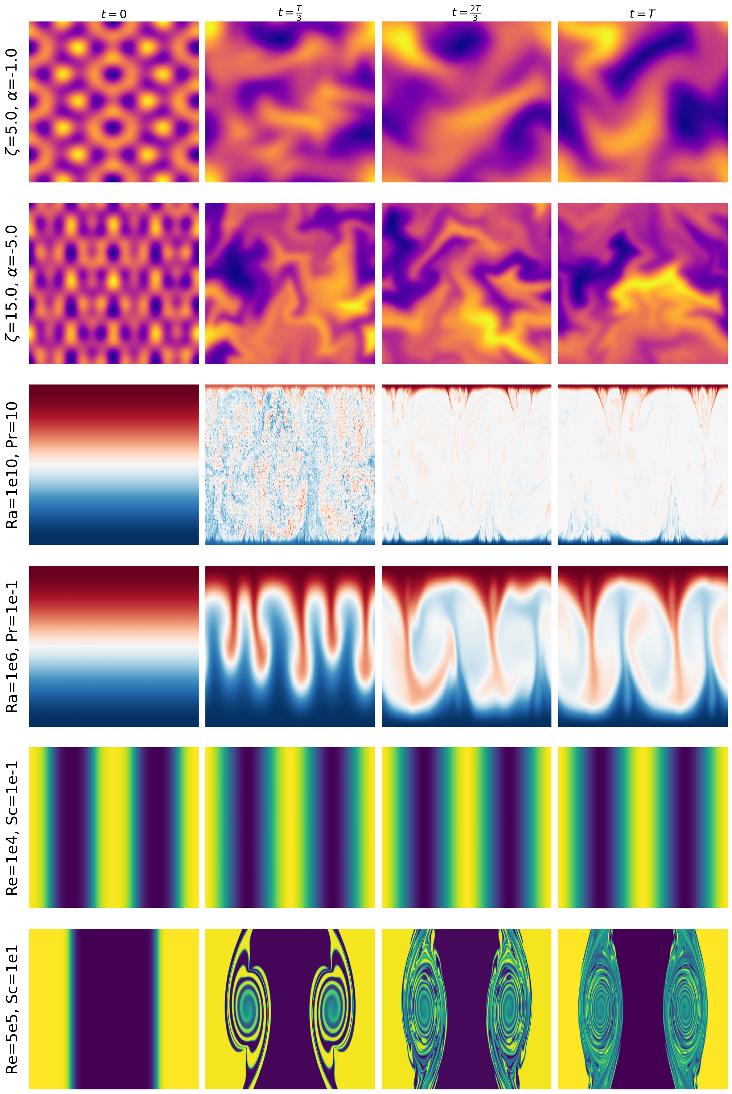
Figure 1 解读：这张图给出三类评估系统的 trajectory examples：active matter、Rayleigh-Bénard convection 和 shear flow。它的作用不是展示模型结构，而是说明任务为什么不同于普通 video SSL：每个样本是多通道物理场随时间演化，空间纹理背后有具体方程和参数。对 JEPA 来说，context-target prediction 的目标不是生成视觉上最锐利的未来帧，而是在压缩表示中保留能区分这些演化机制的状态信息；对下游 probe 来说，若 representation 能恢复参数，就说明它捕获了图中轨迹差异背后的物理原因。

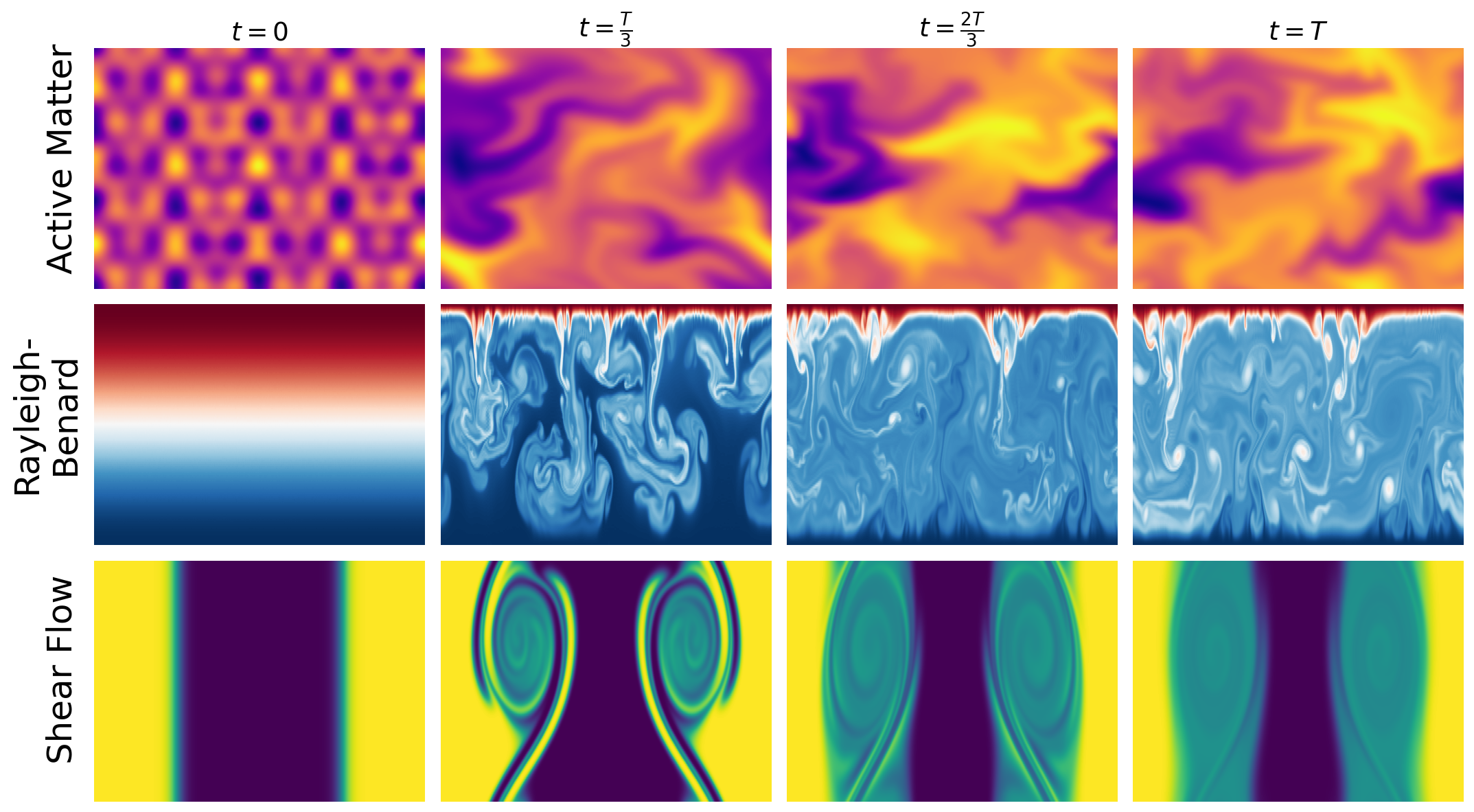
Figure 2 解读：Figure 2 展示同一类系统在不同 physical parameters 下会产生显著不同的演化形态，例如 Rayleigh-Bénard 中不同 Rayleigh / Prandtl number 会改变对流单元与湍动结构。这个图对应论文的 evaluation design：参数不是附加标签，而是决定动力学的 latent cause；因此 parameter prediction MSE 可以作为表征是否物理相关的量化 proxy。

直觉上，JEPA 在这里可能有效，是因为物理系统的高频场值、局部数值误差和可视化纹理并不总是下游任务所需的充分统计量。若强迫模型在 pixel space 中复原未来，会把容量用于低层重建；若强迫它在 latent space 中预测下一个时间块，同时用 variance/covariance regularization 保持非塌缩表示，模型更容易学习到“哪些因素会稳定影响未来演化”。这类因素与 governing parameters 更接近，所以 frozen encoder 上的 probe 更容易回归参数。

3.2 JEPA objective 与 VICReg-style loss

论文把一个含 $T$ 个时间步的样本记作 $x_{0 : T}$ ，把相邻时间块写成 $x_{i}$ 与 $x_{i + 1}$ 。目标是学习 encoder $f : X \to Z$ 和 predictor $g : Z \to Z$ ，最小化： $L (f, g) = E_{x_{i}, x_{i + 1} \sim X} [ℓ_{VICReg} (g (f (x_{i})), f (x_{i + 1}))] .$ VICReg-style loss 写作： $ℓ_{VICReg} (z_{i}, z_{i + 1}) = λ s (z_{i}, z_{i + 1}) + μ [v (z_{i}) + v (z_{i + 1})] + ν [c (z_{i}) + c (z_{i + 1})] .$ 其中 $s$ 是 invariance / similarity criterion，论文用 squared distance 约束预测表示接近 target 表示； $v$ 是 variance regularization，惩罚 batch 内标准差低于阈值的维度，避免 collapse； $c$ 是 covariance regularization，惩罚不同 feature dimensions 的 off-diagonal covariance，鼓励信息分散到多个维度。Appendix B 给出实际超参数 $λ = 2, μ = 40, ν = 2$ ；released code 的 configs/train_shearflow_small.yaml、configs/train_rayleighbenard_small.yaml、configs/train_activematter_small.yaml 中对应 sim_coeff=2、std_coeff=40、cov_coeff=2，因此这里的训练数值来自具体 experiment configs，而不是 base default。

论文公式与 released code 实现差异：论文描述的是 $g (f (x_{i}))$ 与 $f (x_{i + 1})$ 的 latent prediction，并没有强调 mask；当前 code 的 physics_jepa/train_jepa.py 也是 consecutive context/target window prediction，没有 VideoMAE 式随机 tube mask，也没有 EMA target encoder。physics_jepa/model.py 的 get_model_and_loss_cnn() 将 vicreg_loss_3d(..., n_chunks=5) 作为 loss，并在 3D/2D feature chunks 上求均值；这比论文公式更工程化，因为它把空间/时间 feature map 分块后分别计算 loss，降低一次性 covariance 统计的内存压力。

3.3 Encoder / predictor architecture

Appendix B 说明所有 encoder 输入为 $l \times w \times d \times t$ ，其中 $l, w$ 为空间尺寸， $d$ 是物理场通道数， $t = 16$ 是 context frames。JEPA encoder 和 predictor 都是 3D convolutional networks，最终 JEPA encoder 输出为 $l /16 \times w /16 \times 128$ 。released code 中实际训练配置覆盖了默认 configs/model/conv_small.yaml：三个 configs/train_*_small.yaml 都设置 model.dims=[16,32,64,128,128]、num_res_blocks=[3,3,3,9,3]、dataset.num_frames=16。physics_jepa/utils/model_utils.py 中 ConvEncoder 用 3D convolution stem 和 downsample layers 处理时空输入；ConvPredictor 是带 inverse bottleneck 的 CNN，用两层 convolution 从 context embedding 预测 target embedding。

需要注意一个 code-level nuance：configs/dataset/*.yaml 的默认 num_frames 是 4，但实际 JEPA experiment config 在 configs/train_*_small.yaml 中覆盖为 16；因此训练设置应引用 train config，而不是 dataset default。shear flow 与 Rayleigh-Bénard 配置使用 num_chans=4、resolution=224、offset=4；active matter 使用 num_chans=11、resolution=224、offset=1。pretraining launch scripts scripts/*/run_train_jepa.sh 使用 torchrun --nproc_per_node=8 --standalone -m physics_jepa.train_jepa ...，说明 released recipe 期望 8 个 GPU 进程；论文和 repo 没有说明 GPU 型号。

3.4 Dataset windowing and label construction

论文的数据来自 The Well 的三类 PDE-governed systems。released code 的 WellDatasetForJEPA 会遍历每个 HDF5 shard，构建 (file_id, object_id, t0) 索引，使 t0 + 2*num_frames <= T；读取连续 $2 F$ 帧后，把前 $F$ 帧放入 context，后 $F$ 帧放入 target，并将物理参数从 HDF5 scalars 组读出。active matter 忽略常数 L，只预测 $α, ζ$ ；shear flow 与 Rayleigh-Bénard 会调整 channel order，使 velocity/buoyancy/pressure 等通道顺序与模型输入一致。下游 fine-tuning 中，BaseFinetuner 还会对标签做 normalization：active matter 用 means [-3.0, 9.0]、stds [1.41, 5.16]；shear flow 对第一个参数取 log10 后用 means [4.85,2.69]、stds [0.61,3.38]；Rayleigh-Bénard 对第二个参数取 log10 后用 means [2.69,8.0]、stds [3.38,1.41]。

论文公式与 released code 实现差异：当前 physics_jepa/data.py 的 WellDatasetForJEPA.__getitem__ 末尾实际返回 (ctx_t, physical_params, state_labels, bcs) tuple，而 Trainer.step()、JepaTrainer.pred_fn() 和 BaseFinetuner.inference_step() 都按 dict key 访问 batch['context']、batch['target']、batch['physical_params']。文件里保留了一行被注释掉的 dict return。阅读笔记中的伪代码按 trainer 期望的 intended dict interface 写出，同时把这个 current-HEAD mismatch 标为复现 caveat；如果直接运行 main@bb77f7b5，需要先修正 dataset return 或添加 collate/adapter。

3.5 Pseudocode：按 released code 抽象出的关键组件

import torch
import torch.nn.functional as F
from einops import rearrange
 
 
def build_context_target_window(h5_file, file_id, object_id, t0, num_frames=16, resolution=(224, 224)):
    """Intended interface behind physics_jepa.data.WellDatasetForJEPA."""
    raw = read_all_fields(h5_file, object_id, t0, t0 + 2 * num_frames)  # [2F, H, W, C]
    context = raw[:num_frames]
    target = raw[num_frames:]
    context = torch.from_numpy(context).permute(3, 0, 1, 2).contiguous()  # [C, F, H, W]
    target = torch.from_numpy(target).permute(3, 0, 1, 2).contiguous()
    context = F.interpolate(context, size=resolution, mode="bilinear", align_corners=False)
    target = F.interpolate(target, size=resolution, mode="bilinear", align_corners=False)
    physical_params = torch.tensor(read_scalar_parameters(h5_file, file_id))
    return {"context": context, "target": target, "physical_params": physical_params}

import torch
import torch.nn as nn
 
 
class ConvPhysicsJEPA(nn.Module):
    """Condensed from get_model_and_loss_cnn + JepaTrainer.pred_fn."""
    def __init__(self, encoder, predictor, loss_fn):
        super().__init__()
        self.encoder = encoder
        self.predictor = predictor
        self.loss_fn = loss_fn
 
    def forward(self, batch):
        context = batch["context"]  # [B, C, T, H, W]
        target = batch["target"]
        if context.shape[2] < 4:
            context = F.pad(context, (0, 0, 0, 0, 0, 4 - context.shape[2]))
        if target.shape[2] < 4:
            target = F.pad(target, (0, 0, 0, 0, 0, 4 - target.shape[2]))
        ctx_embed = self.encoder(context)
        tgt_embed = self.encoder(target)
        pred_embed = self.predictor(ctx_embed)
        if pred_embed.ndim < 5:
            loss_dict = self.loss_fn(pred_embed.unsqueeze(2), tgt_embed.unsqueeze(2))
        else:
            loss_dict = self.loss_fn(pred_embed, tgt_embed)
        return pred_embed, loss_dict

import torch
import torch.nn.functional as F
 
 
def vicreg_3d_loss(pred, target, sim_coeff=2.0, std_coeff=40.0, cov_coeff=2.0, n_chunks=5):
    """Condensed from physics_jepa.model.vicreg_loss_3d/vicreg_loss."""
    pred_chunks = torch.chunk(pred, n_chunks, dim=0)
    tgt_chunks = torch.chunk(target, n_chunks, dim=0)
    losses = []
    for x, y in zip(pred_chunks, tgt_chunks):
        x = x.flatten(1)
        y = y.flatten(1)
        repr_loss = F.mse_loss(x, y)
        std_x = torch.sqrt(x.var(dim=0) + 1e-4)
        std_y = torch.sqrt(y.var(dim=0) + 1e-4)
        std_loss = torch.mean(F.relu(1.0 - std_x)) + torch.mean(F.relu(1.0 - std_y))
        x = x - x.mean(dim=0)
        y = y - y.mean(dim=0)
        cov_x = (x.T @ x) / max(x.shape[0] - 1, 1)
        cov_y = (y.T @ y) / max(y.shape[0] - 1, 1)
        cov_loss = off_diagonal(cov_x).pow(2).sum() / x.shape[1]
        cov_loss = cov_loss + off_diagonal(cov_y).pow(2).sum() / y.shape[1]
        losses.append(sim_coeff * repr_loss + std_coeff * std_loss + cov_coeff * cov_loss)
    return torch.stack(losses).mean()

import torch
import torch.nn as nn
 
 
class FrozenEncoderParameterProbe(nn.Module):
    """Condensed from BaseFinetuner/JepaFinetuner."""
    def __init__(self, encoder, attentive_head, label_stats):
        super().__init__()
        self.encoder = encoder.eval()
        for p in self.encoder.parameters():
            p.requires_grad = False
        self.head = attentive_head
        self.label_stats = label_stats
        self.loss_fn = nn.MSELoss()
 
    def forward(self, batch):
        with torch.no_grad():
            z = self.encoder(batch["context"])
            z = rearrange(z, "b c h w -> b (h w) c")
        labels = normalize_labels(batch["physical_params"], stats=self.label_stats)
        pred = self.head(z)
        return {"loss": self.loss_fn(pred, labels), "pred": pred}

3.6 Code-to-paper mapping

Code reference: main @ bb77f7b5 (2026-03-18) — pseudocode and mapping based on this commit

Paper Concept	Source File	Key Class/Function
JEPA context-target latent prediction	`physics_jepa/train_jepa.py`	`JepaTrainer.pred_fn`
JEPA encoder/predictor construction	`physics_jepa/model.py`, `physics_jepa/utils/model_utils.py`	`get_model_and_loss_cnn`, `ConvEncoder`, `ConvPredictor`
VICReg-style objective	`physics_jepa/model.py`	`vicreg_loss_3d`, `vicreg_loss`
Optional Gaussian matching loss not used by normal configs	`physics_jepa/model.py`, `physics_jepa/train.py`	`BCS`, `vicreg_loss_bcs`, `cfg.model.loss == "gaussian_matching"`
The Well HDF5 trajectory windows and physical parameters	`physics_jepa/data.py`	`WellDatasetForJEPA`, `get_train_dataloader_from_cfg`
Frozen encoder parameter-estimation probes	`physics_jepa/finetuner.py`, `physics_jepa/finetune.py`	`BaseFinetuner`, `JepaFinetuner`, `VideoMAEFinetuner`
VideoMAE baseline feature extraction	`physics_jepa/videomae.py`, `physics_jepa/finetuner.py`	`vit_small_patch16_224`, `VideoMAEFinetuner`
DISCO / MPP baselines	`physics_jepa/baselines/disco.py`, `physics_jepa/baselines/mpp_param_estimation.py`	DISCO embedding loader, `ParameterEstimationModel`
Actual launch/config values	`scripts//run_train_jepa.sh`, `configs/train__small.yaml`	8-process torchrun, 16 frames, AdamW/cosine, `sim/std/cov` coefficients

4. Experimental Setup (实验设置)

Datasets and scale. 论文使用 The Well 中三个 2D physical simulation datasets，并在每个系统上做 physical parameter prediction。The Well overview 给出的规模是：active_matter 为 $256 \times 256$ resolution、81 time steps、360 trajectories、约 51.3GB；shear_flow 为 $128 \times 256$ 、200 time steps、1,120 trajectories、约 115GB；

rayleigh_benard 为 $512 \times 128$ 、200 time steps、1,750 trajectories、约 358GB。The Well 的常规 split 是 train/test/validation = 0.8/0.1/0.1。论文自身没有列出每个 split 的窗口样本总数；唯一明确的 fine-tuning example 数字是 shear flow 中 50% fine-tuning data = 16k examples，因此 100% fine-tuning set 对应约 32k examples。

released code 会根据 num_frames=16 与 dataset-specific offset 在 HDF5 中动态生成 windowed examples，并在运行时打印 batch/window 数。

Systems and target parameters. Active matter 模拟 rodlike active particles in a Stokes fluid，目标参数是 $α$ 与 $ζ$ 。Rayleigh-Bénard convection 模拟底部加热、顶部冷却的水平流体层，目标参数是 Rayleigh number 与 Prandtl number；论文文字中把 Rayleigh number 记作 $ν$ ，但物理含义是 buoyancy forces 与 viscous forces 的比值。Shear flow 描述平行流体层之间的边界与涡旋/湍流形成，目标参数是 Reynolds number 与 Schmidt number。

Baselines. 比较对象分成两类：self-supervised representation learning 包括 JEPA 和 VideoMAE；physical modeling baselines 包括 DISCO 与 MPP。VideoMAE 是 masked autoencoder with pixel-level reconstruction objective，论文中使用 VideoMAE ViT-tiny/16 并从 scratch pretrain。DISCO 是 in-context operator learning / latent operator 方法，用预训练模型输出的 latent representation 做 probe。MPP 是 Multiple Physics Pretraining 的 autoregressive foundation model，实验用 published pretrained AViT-tiny weights，并做 end-to-end fine-tuning，因为 MPP pretraining 不包含这三个目标数据集。

Evaluation metric. 主指标是 physical parameter prediction MSE，lower is better。论文报告每个系统两个 governing parameters 的 averaged MSE：active matter 平均 $α, ζ$ ；shear flow 平均 Reynolds、Schmidt；Rayleigh-Bénard 平均 Rayleigh、Prandtl。released code 在 fine-tuning 前会对物理参数做 normalization，部分参数先取 $lo g_{10}$ 再标准化，所以 table 数字应理解为该 pipeline 下的参数回归 MSE，而不是原始物理单位上的绝对误差。

Training config. Appendix B 写明所有 encoder 输入 16 context frames，JEPA encoder 输出 $l /16 \times w /16 \times 128$ ，VideoMAE small ViT patch size 16 的输出为 $l /16 \times w /16 \times t /2 \times 384$ ，DISCO embedding 为 $1 \times 384$ ，MPP embedding 为 $l /16 \times w /16 \times 192$ 。JEPA 和 VideoMAE pretrain 6 epochs；所有模型 fine-tune 100 epochs；

训练和 fine-tuning 都用 AdamW optimizer + cosine learning-rate schedule。released JEPA configs 补充了具体数值：shear flow 用 configs/train_shearflow_small.yaml，num_epochs=6、batch_size=8 per device、lr=1e-4、weight_decay=0.05、warmup 6 epochs、noise_std=1.0、ft.batch_size=64、ft.num_train_steps=320、ft.num_val_steps=150；

Rayleigh-Bénard 用 configs/train_rayleighbenard_small.yaml，num_epochs=30、batch_size=8、lr=1e-4、warmup 6 epochs、fine-tune LR 1e-3；active matter 用 configs/train_activematter_small.yaml，num_epochs=30、batch_size=8、lr=1e-3、warmup 2 epochs、noise_std=1.0。

这里存在 paper-vs-code difference：论文 Appendix B 概括说 JEPA/VideoMAE pretrain 6 epochs，但 current code 的 rayleigh_benard 与 active_matter JEPA configs 写的是 30 epochs；note 以论文为主报告实验设置，同时明确记录 released code 的实际 config。

5. Experimental Results (实验结果)

Main parameter-estimation results. Table 1 的 MSE 数字如下：

Method	Active matter	Shear flow	Rayleigh-Bénard convection
JEPA	0.079	0.38	0.13
VideoMAE	0.160	0.67	0.18
DISCO	0.057	0.13	0.01
MPP (full finetuning)	0.230	0.59	0.08

这些结果支持两个结论。第一，在同样作为 generic SSL 的比较中，JEPA 全面优于 VideoMAE：active matter 从 0.160 降到 0.079，相对提升约 51%；shear flow 从 0.67 降到 0.38，相对提升约 43%；Rayleigh-Bénard 从 0.18 降到 0.13，相对提升约 28%。这说明 latent-space prediction 比 masked pixel reconstruction 更能保留 governing parameters。第二，physics-specific 方法并不总是稳胜 generic SSL：DISCO 最强，尤其 Rayleigh-Bénard 达到 0.01；但 MPP 即使 full fine-tuning 也在 active matter 上为 0.230、shear flow 上为 0.59，均弱于 JEPA。这与论文的解释一致：autoregressive pixel-level surrogate 对 non-generative downstream tasks 可能不是最合适的 representation learner。

Data scaling / sample efficiency. Table 2 在 shear flow 参数预测上比较 fine-tuning dataset fraction：

Method	10%	50%	100%
JEPA	0.57	0.40	0.38
VideoMAE	0.98	0.75	0.67

JEPA 的 scaling 更好：只用 50% fine-tuning data（论文写明为 16k examples）时，MSE = 0.40，已经达到 100% data 时 0.38 的约 95% performance；10% data 时的 0.57 也优于 VideoMAE 在 100% data 下的 0.67。这个结果对应用很关键，因为真实科学数据往往有大量 unlabeled trajectories，但高质量参数标注、实验条件或反问题标签可能很少。JEPA 的 frozen representation 更 sample-efficient，说明预训练阶段已经把更多参数相关信息压进 embedding。

Latent prediction vs pixel-level prediction. 论文把 DISCO 和 JEPA 视为各自类别中最好的 latent prediction/latent operator 方法，把 MPP 和 VideoMAE 视为更接近 pixel-level 或 autoregressive prediction 的方法。Table 1 中 DISCO 与 JEPA 在 active matter 上接近（0.057 vs 0.079），但在 Rayleigh-Bénard 上差一个数量级（0.01 vs 0.13）；VideoMAE 在 Rayleigh-Bénard 上与 JEPA 的差距最小（0.18 vs 0.13）。这说明“latent space 更好”不是一个无条件定理，系统特性、模型归纳偏置和预训练数据覆盖都会影响结果；但在这三个测试系统上，latent representation learning 的趋势清晰强于 pixel reconstruction/autoregressive surrogate。

Ablation status. 论文没有提供传统意义上的 component ablation，例如去掉 covariance loss、替换 predictor 深度、改变 encoder capacity、改变 $λ, μ, ν$ 的系统表格。最接近 ablation 的是 Table 2 的 fine-tuning data fraction study，它证明 JEPA 表征在 labeled data scarcity 下更稳。Appendix B 只说明经验上 $λ = 2, μ = 40, ν = 2$ 表现较好，没有给出不同系数的对比曲线。因此复现或扩展时，最应该补的实验是 VICReg terms、context length、target horizon、encoder scale、dataset noise 和 cross-system transfer 的消融。

Limitations and caveats. 作者结论强调 latent-space predictive learning 可作为 scientific ML 的 promising foundation，但当前 paper scope 较窄：只测试三个 2D The Well 系统，主要下游任务是参数估计，没有验证 long rollout、control、out-of-distribution parameter ranges、跨系统 pretraining 或真实实验数据。

公开代码也有复现 caveat：main@bb77f7b5 的 dataset return 与 trainer/finetuner 期望的 dict interface 不一致；VideoMAE pretraining 的完整 launch recipe 在 repo 中不如 JEPA 清晰；GPU type 与部分 dataset split/window count 没有在 paper 或 repo 中完整列出。

结论应谨慎表述为：在这组 benchmark 与实现设置下，JEPA-style latent prediction 学到的表示比 pixel-level MAE / autoregressive MPP 更适合 physical parameter estimation，但它还不是一个完整的 physical world model 或 PDE surrogate replacement。

Paper Notes

探索

Representation Learning for Spatiotemporal Physical Systems

Representation Learning for Spatiotemporal Physical Systems

1. Motivation (研究动机)

2. Idea (核心思想)

3. Method (方法)

3.1 Overall framework：从轨迹窗口到参数估计

3.2 JEPA objective 与 VICReg-style loss

3.3 Encoder / predictor architecture

3.4 Dataset windowing and label construction

3.5 Pseudocode：按 released code 抽象出的关键组件

3.6 Code-to-paper mapping

4. Experimental Setup (实验设置)

5. Experimental Results (实验结果)

目录