SANA-Video: Efficient Video Generation with Block Linear Diffusion Transformer

Paper: arXiv:2509.24695v2 · DOI · NVIDIA EAI page Code: NVlabs/Sana · SANA-Video docs Code reference: main @ 6554c8d9 (2026-05-16) — pseudocode、config 数字与 mapping 基于该 released code 快照；GitHub default branch main 于 2026-05-18 仍指向该 SHA。 Authors: Junsong Chen*, Yuyang Zhao*, Jincheng Yu*, Ruihang Chu, Junyu Chen, Shuai Yang, Xianbang Wang, Yicheng Pan, Daquan Zhou, Huan Ling, Haozhe Liu, Hongwei Yi, Hao Zhang, Muyang Li, Yukang Chen, Han Cai, Sanja Fidler, Ping Luo, Song Han, Enze Xie Affiliations: NVIDIA, HKU, MIT, THU, PKU, KAUST Venue: ICLR 2026 Oral

1. Motivation (研究动机)

1.1 视频生成的计算瓶颈

当前视频生成模型面临严重的 计算效率 问题: Token 数量巨大: 以 Wan 14B 为例, 生成一个 720p 5 秒视频需要处理超过 75,000 个 token, 在 H100 GPU 上需要 32 分钟 Self-attention 的二次复杂度: 传统 self-attention 的 $O (N^{2})$ 复杂度在视频生成的大量 token 场景下成为主要瓶颈 长视频生成更加困难: 超过 10 秒的长视频因为 full-sequence processing 和 KV cache 的线性增长, 几乎无法用现有模型实现 训练成本高昂: MovieGen 等大模型需要巨量 GPU 资源, 限制了研究社区的参与这篇论文的动机不是单纯“把模型做小”，而是把视频生成中最昂贵的两项同时压下来：第一，DiT 在空间-时间 token 上做 full self-attention，长宽、帧数、denoising step 任一维度增长都会放大 attention 成本；

第二，若直接把长视频写成 autoregressive blocks，普通 causal attention 的 KV cache 仍会随历史长度线性增长。SANA-Video 的目标因此是一个端到端效率问题：短视频要能在单卡上快速生成，长视频要能携带全局历史而不让缓存占满显存。论文给出的效率约束很具体：模型需要覆盖 $720 \times 1280$ 高分辨率、81-frame / 5s 常用生成设置，并进一步延伸到 minute-length 视频；部署侧不只面向 H100，也要能在 RTX 5090 上通过 NVFP4 量化运行。这样的设定使“训练成本”“推理延迟”“显存缓存”变成同一个架构问题，而不是独立的工程优化。

1.2 现有方法的局限

Causal Full Attention: 内存 $O (N \times D)$ , 计算 $O (N^{2} \times D)$ , 无法支持长视频 Causal Local Attention: 虽然降低了计算量到 $O (N \times W \times D)$ , 但丧失了 global context 信息 KV Cache 方案: 传统 KV cache 随序列长度线性增长, 内存开销大

局部注意力的关键损失是“看不到全局历史”：它能让每个 block 的显存可控，但对于跨镜头身份一致性、动作连续性和 long-range prompt adherence，它只能依赖有限窗口。SANA-Video 试图保留全局历史，但把历史压缩成 linear attention 的累积状态；这个状态的大小与时间长度无关，只与 head dimension 相关。

1.3 核心问题

Can we develop a high-quality and high-resolution video generator that is computationally efficient and runs very fast on both cloud and edge devices?

2. Idea (核心思想)

SANA-Video 提出了一个 小型但高效的 diffusion model (2B 参数), 通过两个核心设计实现高效视频生成:

Linear DiT: 用 linear attention (ReLU kernel + RoPE) 替代传统 self-attention, 将复杂度从 $O (N^{2})$ 降到 $O (N)$ , 实现 4x 加速
Block Linear Attention with Constant-Memory KV Cache: 利用 linear attention 的累积性质, 设计 constant-memory 的 KV cache, 支持分块自回归生成分钟级长视频
高效训练策略: 从 SANA T2I 模型 continue pre-training, 结合高效数据过滤, 进一步降低训练成本

核心 insight 可以概括为：如果 attention kernel 允许把历史写成 $\sum K^{⊤} V$ 与 $\sum K$ 这样的可累加状态，那么长视频不必保存每个历史 token 的 KV；只要当前 block 的 query 能读这个累计状态，就能以固定内存获得全局上下文。与普通 linear attention 不同，SANA-Video 还要解决视频位置编码和 temporal locality，因此把 3D RoPE 放在 ReLU kernel 之后，并在 Mix-FFN 中补入 spatial-temporal convolution。

与 Wan / SkyReels 等小型 video DiT 的主要差异是：后者通常仍依赖 full attention 或局部/窗口化 attention，在高 token 数和长历史下必须在质量、窗口长度、显存之间折中；SANA-Video 的 Linear DiT 把短视频的主要 attention 成本降下来，LongSANA 再用 block causal linear state 把历史缓存变成常数级。换言之，本文不是一个 sampler-only 加速方法，而是把 backbone attention、block inference cache、VAE 压缩和数据过滤连成一套低成本生成系统。

3. Method (方法)

3.1 整体架构

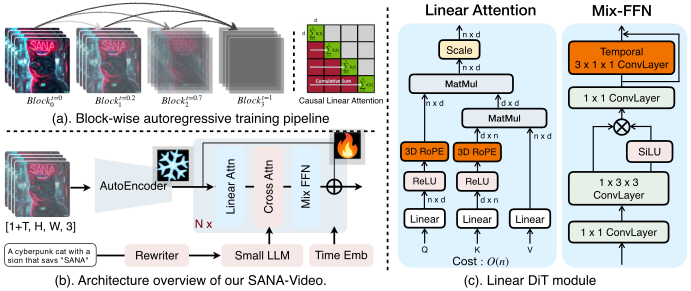
Figure 2 解读: 这是 SANA-Video 的整体架构图。(a) 展示了基于 block causal KV cache 的分块自回归训练 pipeline。(b) 展示了模型的完整 pipeline: 输入视频经过 AutoEncoder 编码为 latent, 文本经过 Rewriter → Small LLM 处理, 然后通过 N 个 Transformer block (包含 Linear Attention, Cross Attention, Mix-FFN) 进行去噪。(c) 展示了 Linear DiT module 的详细设计: Q, K, V 经过 Linear projection 和 ReLU 激活后, 对 Q 和 K 分别应用 3D RoPE, 然后通过 MatMul 计算注意力; Mix-FFN 部分包含 1x3x3 spatial ConvLayer 和 3x1x1 temporal ConvLayer, 总计算成本为 $O (n)$ 。

3.2 Linear Attention with RoPE

问题: 将 RoPE 集成到 Linear Attention

直接在 linear attention 中使用 RoPE 会导致数值不稳定 — softmax 和 ReLU similarity function 的差异使得 RoPE 变换可能让分母趋向零。

解决方案: RoPE(ReLU(x)) 而非 RoPE(x)

核心思想: 先 ReLU 再 RoPE, 确保分母中不含 RoPE (分母只对 key 做 $ϕ (K)$ 求和), 保持非负性:

O_{i} = \frac{RoPE ( ϕ ( Q _{i} )) ( \sum _{j = 1}^{N} RoPE ( ϕ ( K _{j} ) ) ^{T} V _{j} )}{ϕ ( Q _{i} ) ( \sum _{j = 1}^{N} ϕ ( K _{j} ) ^{T} )}

其中 $ϕ (\cdot) = ReLU (\cdot)$ 。分子中 Q 和 K 都有 RoPE 用于位置编码, 分母中去掉 RoPE 保证数值稳定性。

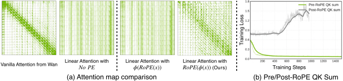
Figure 3 解读: (a) 比较了不同 attention map: Wan 的 vanilla softmax attention 具有清晰的局部模式; 无 PE 的 linear attention 过于 dense; $ϕ (RoPE (x))$ 先 RoPE 后 ReLU 的结果也较密集; 而本文的 $RoPE (ϕ (x))$ 先 ReLU 后 RoPE 产生了更稀疏、更聚焦局部区域的注意力模式。(b) Pre/Post-RoPE QK sum 的训练 loss 对比, 从分母中去掉 RoPE (绿线) 保证了训练稳定性。

#Pseudocode: Linear Attention with RoPE
def linear_attention_with_rope(Q, K, V, rope_freqs):
    """
    Q, K, V: (B, N, H, D)  # batch, seq_len, heads, dim
    rope_freqs: 3D rotary position embeddings
    """
    # Step 1: ReLU activation (kernel function phi)
    Q_relu = relu(Q)  # phi(Q)
    K_relu = relu(K)  # phi(K)
 
    # Step 2: Apply 3D RoPE AFTER ReLU
    Q_rope = apply_3d_rope(Q_relu, rope_freqs)  # RoPE(phi(Q))
    K_rope = apply_3d_rope(K_relu, rope_freqs)  # RoPE(phi(K))
 
    # Step 3: Compute numerator with RoPE (positional encoding)
    # sum_j RoPE(phi(K_j))^T V_j  -> (B, H, D, D)
    KV = einsum('bnhd, bnhe -> bhde', K_rope, V)
    numerator = einsum('bnhd, bhde -> bnhe', Q_rope, KV)
 
    # Step 4: Compute denominator WITHOUT RoPE (numerical stability)
    # sum_j phi(K_j)^T  -> (B, H, D)
    K_sum = K_relu.sum(dim=1)  # no RoPE here!
    denominator = einsum('bnhd, bhd -> bnh', Q_relu, K_sum)
 
    # Step 5: Normalize
    output = numerator / (denominator.unsqueeze(-1) + eps)
    return output

代码映射: diffusion/model/nets/sana_blocks.py 中的 LiteLAReLURope 类实现了此机制。

3.3 Mix-FFN with Spatial-Temporal Convolution

Linear attention 的 attention map 较 dense, 缺乏局部关注能力。Mix-FFN 通过 convolution 弥补这一不足:

Spatial Conv: 1x3x3 ConvLayer 捕获空间局部特征 Temporal Conv: 3x1x1 ConvLayer (shortcut connection) 捕获时间维度的局部关系 Temporal conv 采用 zero-initialized shortcut, 不影响预训练权重

#Pseudocode: Spatial-Temporal Mix-FFN
def mix_ffn(x, T, H, W):
    """
    x: (B, T*H*W, D)  # flattened video tokens
    """
    # 1x1 conv (linear projection up)
    x_up = conv1x1_up(x)  # (B, T*H*W, 4D)
 
    # Reshape to 3D for convolutions
    x_3d = x_up.reshape(B, T, H, W, 4*D)
 
    # Spatial 1x3x3 convolution
    x_spatial = depthwise_conv3x3(x_3d)  # spatial local features
    x_spatial = silu(x_spatial)
 
    # Temporal 3x1x1 convolution with shortcut
    x_temporal = temporal_conv(x_3d)  # temporal local features
    x_out = x_spatial + x_temporal  # shortcut connection
 
    # 1x1 conv (linear projection down)
    output = conv1x1_down(x_out)  # (B, T*H*W, D)
    return output

代码映射: sana_blocks.py 中的 GLUMBConvTemp 类; temporal conv 通过 t_kernel_size 参数控制。

3.4 Block Linear Attention with Constant-Memory KV Cache

这是支持长视频生成的核心创新。

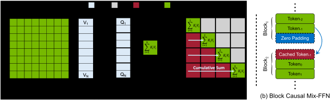
Figure 4 解读: (a) 对比了三种 attention 的计算机制: Vanilla Attention 需要完整的 $N \times N$ attention matrix 和 $N \times D$ 的 KV cache; Linear Attention 将 K, V 先做外积再与 Q 相乘, 复杂度降为 $O (D^{2})$ ; Causal Linear Attention 维护 cumulative sum $\sum K V$ , 每个新 token 只需 $O (D^{2})$ 的计算和固定内存。(b) Block Causal Mix-FFN 的处理方式: 在相邻 block 之间, 缓存上一个 block 的最后一个 token (Cached Token_{-1}), 并在当前 block 开头添加 Zero Padding, 确保 temporal convolution 的因果性。

Causal Linear Attention 的 KV Cache 重新推导

对于第 $i$ 个 token 的 causal linear attention 输出:

O_{i} = \frac{ϕ ( Q _{i} ) ( \sum _{j = 1}^{i - 1} S _{j} + S _{i} )}{ϕ ( Q _{i} ) ( \sum _{j = 1}^{i - 1} ϕ ( K _{j} ) ^{T} + ϕ ( K _{i} ) ^{T} )}

其中 $S_{j} = ϕ (K_{j})^{T} V_{j}$ 是 attention state。关键洞察: 只需存储: Cumulative sum of states: $\sum_{j = 1}^{i - 1} S_{j} \in R^{D \times D}$ Cumulative sum of keys: $\sum_{j = 1}^{i - 1} ϕ (K_{j})^{T} \in R^{D \times 1}$

内存成本为 $O (D^{2})$ , 与序列长度 N 无关!

Metric	Causal Full Attention	Causal Local Attention	Causal Linear Attention
Memory	$O (N \times D)$	$O (W \times D)$	$O (D^{2})$
Comp. Cost (N-th token)	$O (N \times D)$	$O (W \times D)$	$O (D^{2})$
Comp. Cost (N tokens)	$O (N^{2} \times D)$	$O (N \times W \times D)$	$O (N \times D^{2})$
Global Context	Yes	No	Yes

#Pseudocode: Block Linear Attention Inference with KV Cache
def block_linear_inference(model, num_blocks, denoise_timesteps, noise_scheduler):
    """
    Algorithm 1 from the paper.
    KV cache stores: [sum_S, sum_phi_K, conv_cache_f]
    """
    kv_cache = [None, None, None]  # cumulative_S, cumulative_K, conv_cache
    output_blocks = []
 
    for i in range(num_blocks):  # M blocks
        # Initialize noise for this block
        x_noisy = sample_noise(shape)  # x^i_{t_T} ~ N(0, I)
 
        for j in reversed(range(len(denoise_timesteps))):  # T -> 1 denoising
            # Forward pass with KV cache
            x_denoised = model(x_noisy, denoise_timesteps[j], kv_cache)
 
            if j == 0:  # Last denoising step (fully denoised)
                output_blocks.append(x_denoised)
                # Update KV cache with this block's information
                # sum_S += phi(K_block)^T @ V_block
                # sum_phi_K += sum(phi(K_block))
                # conv_cache = last_token_of_block
                kv_cache = update_kv_cache(model, x_denoised, kv_cache)
            else:
                # Self-forcing: add noise to denoised output
                epsilon = sample_noise(shape)
                x_noisy = noise_scheduler(x_denoised, epsilon, denoise_timesteps[j-1])
 
    return concat(output_blocks)

代码映射: diffusion/model/nets/sana_multi_scale_video.py 中的 forward_long() 方法; diffusion/model/nets/sana_blocks.py 中的 CachedCausalAttention 和 CachedGLUMBConvTemp。

Block Causal Mix-FFN

为了保证 temporal conv 的因果性:

训练时: 在每个 block 末尾 append 一个 all-zero token (Zero Padding), 防止信息泄露
推理时: 缓存上一个 block 的 最后一个 token (Token_{-1}), prepend 到当前 block 开头, 为 causal temporal convolution (kernel size 3) 提供前一个 block 的上下文

3.5 训练策略

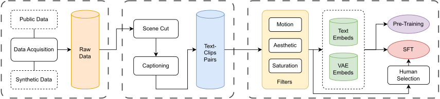
Figure 5 解读: SANA-Video 的数据过滤 pipeline。从 Public Data 和 Synthetic Data 收集原始数据, 经过 Scene Cut 切分为短片段, 使用 Captioning (Qwen-2.5-VL-7B) 生成详细描述 (80-100 words), 然后通过 Motion (Unimatch/VMAF), Aesthetic (DOVER), Saturation (OpenCV) 三个维度进行过滤。最终的高质量数据用于 Pre-Training 和 SFT, SFT 阶段还包含 Human Selection 的约 5,000 个高质量视频。

Stage 1: VAE Adaptation (T2I)

480P: 使用 Wan-VAE (F8T4C16) 720P: 使用自研 DCAE-V (F32T4C32), spatial 下采样 32x, temporal 下采样 4x VAE adaptation 仅需 5-10k steps 即可收敛

Stage 2: Continue Pre-Training from T2I

从 SANA 1.6B T2I 模型初始化新增层 (temporal conv, 3D RoPE) zero-initialized, 保留预训练权重 Coarse-to-fine 训练: 先低分辨率短视频 (192P 2.5s) → 再高分辨率长视频 (480P 5s)

Stage 3: Autoregressive Block Training (LongSANA)

两阶段:

Monotonically Increasing SNR Sampler: 后续 block 的 timestep 单调递增 (即 noise level 更低), 比随机采样收敛更快
Improved Self-Forcing: 利用 block linear attention 的 constant memory 特性, 可以 self-generate 更长视频 (如 1 min), 减少 training-inference gap

3.6 Deep Compression Video Autoencoder (DCAE-V)

Autoencoder	Ratio	PSNR	SSIM	LPIPS
Wan2.1-VAE (F8T4C16)	16	34.41	0.95	0.01
Wan2.2-VAE (F16T4C48)	21	35.61	0.96	0.01
LTX-VAE (F32T8C128)	64	32.26	0.93	0.04
DCAE-V (F32T4C32)	128	33.25	0.94	0.03

DCAE-V 的压缩比高达 128x, 但重建质量与竞品相当。32 个 latent channels 与 T2I 模型对齐, 便于 continue pre-training。

3.7 Released Code 对照与实现核查

Code reference: main @ 6554c8d9 (2026-05-16) — pseudocode and mapping based on this commit.

Paper Concept	Source File	Key Class/Function
SANA-Video backbone / 2B video DiT	`diffusion/model/nets/sana_multi_scale_video.py`	`SanaMSVideo`, `SanaVideoMSBlock`, `SanaMSVideo_2000M_P1_D20`, `SanaMSVideo_2000M_P2_D20`
Linear attention with ReLU + RoPE	`diffusion/model/nets/sana_multi_scale_video.py`, `diffusion/model/nets/sana_blocks.py`	`attn_type="LiteLAReLURope"`, `LiteLAReLURope`, `ChunkedLiteLAReLURope`
Triton fast linear attention kernels	`diffusion/model/nets/fastlinear/modules/lite_mla.py`, `diffusion/model/nets/fastlinear/modules/triton_lite_mla.py`	`LiteMLA`, `TritonLiteMLA`, `linear_relu_fwd`, `pad_vk_mm_fwd`, `vk_q_mm_divide_fwd`
Spatial-temporal Mix-FFN	`diffusion/model/nets/sana_multi_scale_video.py`, `diffusion/model/nets/basic_modules.py`, `diffusion/model/nets/fastlinear/modules/mb_conv_pre_glu.py`	`ffn_type="GLUMBConvTemp"`, `TritonMBConvPreGLU`, temporal kernel `t_kernel_size`
480p training config	`configs/sana_video_config/Sana_2000M_480px_AdamW_fsdp.yaml`	`SanaMSVideo_2000M_P2_D20`, `WanVAE`, `vae_latent_dim=16`, `num_frames=81`
720p LTX2/DCAE-style config	`configs/sana_video_config/Sana_2000M_720px_ltx2vae_AdamW_fsdp.yaml`	`SanaMSVideo_2000M_P1_D20`, `LTX2VAE_diffusers`, `vae_latent_dim=128`, `num_frames=81`
LongSANA block training	`configs/sana_video_config/longsana/480ms/longsana.yaml`, `train_video_scripts/train_longsana.py`	`trainer: longsana`, `num_frame_per_block: 10`, `LongSANATrainer`
Inference / refiner pipeline	`diffusion/longsana/sana_video_pipeline.py`, `app/sana_video_refiner_pipeline_diffusers.py`	`LongSANAVideoInference`, SANA-Video + LTX2 Refiner two-stage pipeline

代码核查的要点：

released config 中 480p 与 720p 都使用 attn_type: LiteLAReLURope 与 ffn_type: GLUMBConvTemp，与论文“Linear DiT + temporal Mix-FFN”的叙述一致。480p 配置使用 SanaMSVideo_2000M_P2_D20 + WanVAE + vae_latent_dim: 16；720p 配置使用 SanaMSVideo_2000M_P1_D20 + LTX2VAE_diffusers + vae_latent_dim: 128。

这说明高分辨率路径不是简单放大 480p VAE，而是换成更高压缩/不同 latent channel 的 VAE 路径。训练 config 给出的关键数值为 train_batch_size: 1, train_batch_size_image: 4, num_epochs: 10, gradient_clip: 0.1, AdamW lr: 5.0e-5, mixed_precision: bf16, use_fsdp: true；这些数字来自 SANA-Video 专用 yaml，不是 base default。

LongSANA config 显式设置 trainer: longsana, lr: 1.0e-05, num_frame_per_block: 10, update_kv_cache_by_end: false，对应论文的 block autoregressive training / self-forcing 路径。论文公式与 released code 实现差异：本次核查没有发现会改变核心算法解释的明显冲突；

需要注意的是 docs 中的 720p public training command 使用 Sana_2000M_720px_ltx2vae_AdamW_fsdp.yaml，而论文正文把 720p 高压缩路径称为 DCAE-V，笔记中保留“论文 DCAE-V / docs config LTX2VAE_diffusers”这一区分，避免把两个命名强行合并。

4. Experimental Setup (实验设置)

4.1 模型配置

Model	Width	Depth	FFN	Heads	Param
SANA-Video-2B	2240	20	6720	20	2056M

Backbone: 基于 SANA 架构, FFN 从 5600 增加到 6720, head dimension 从 32 增加到 112 以适配 3D RoPE Text Encoder: 小型 decoder-only LLM 训练: AdamW optimizer, weight decay 0.03, learning rate 5e-5, Accelerate FSDP 硬件: 64 H100 GPUs, 约 12 天 公开 code config (480p): configs/sana_video_config/Sana_2000M_480px_AdamW_fsdp.yaml 使用 SanaMSVideo_2000M_P2_D20, image_size: 480, num_frames: 81, WanVAE, vae_latent_dim: 16, attn_type: LiteLAReLURope, ffn_type: GLUMBConvTemp, pos_embed_type: wan_rope。

公开 code config (720p): configs/sana_video_config/Sana_2000M_720px_ltx2vae_AdamW_fsdp.yaml 使用 SanaMSVideo_2000M_P1_D20, image_size: 720, num_frames: 81, LTX2VAE_diffusers, vae_latent_dim: 128，并从 hf://Efficient-Large-Model/SANA-Video_2B_720p/... 初始化。

LongSANA config: configs/sana_video_config/longsana/480ms/longsana.yaml 使用 trainer: longsana, lr: 1.0e-05, num_frame_per_block: 10；该配置对应 minute-scale autoregressive blocks，而不是普通 5s T2V 训练。

4.2 Evaluation

Benchmark: VBench (Total Score, Quality, Semantic/I2V) Efficiency Metric: 480P 81-frame 视频的生成延迟 Ablation: training loss curves + H100 latency profiles 720p evaluation: 额外报告 $720 \times 1280 \times 81$ 设定下的 H100 latency 与 VBench。 Autoencoder evaluation: 在 Panda-70M 192p resolution 上比较重建 PSNR / SSIM / LPIPS，并在噪声扰动 $ϵ = 0, 0.1, 0.2$ 下比较 VAE 鲁棒性。 Long video evaluation: LongSANA 与 Self-Forcing、SkyReels-V2、CausVid 等 autoregressive video generation 方法比较；论文还报告 4-step LongSANA 在 H100 上 35s 生成 1-min 16FPS 480P video。

4.3 数据与过滤设置

论文没有给出完整 pre-training 数据集总 clip 数，因此不能把“public + synthetic data”误写成一个具体规模。可确认的信息如下：

Raw source: public real videos + synthetic videos。Scene cutting: 使用 PySceneDetect / FFmpeg 切成 single-scene 5-second clips；pre-training 聚焦 5s、16FPS、单场景视频。Caption rewrite: 使用 Qwen-2.5-VL-7B 生成/重写 prompt，使 prompt 与 clip 对齐；对 synthetic data，重写 prompt 还能降低原 prompt 与生成视频之间的错配。

Motion filtering: 使用 Unimatch optical flow 与 VMAF / FFmpeg pixel difference；每 0.5s 抽帧、resize 到 $320 \times 576$ ，按 source 分别设 motion range，避免过慢或过快运动。Aesthetic filtering: 使用 DOVER 的 overall score 过滤低质量视频。Saturation filtering: 使用 OpenCV 将 RGB 转 HSV，统计 S channel 平均值；过滤高 saturation / HDR-to-SDR 异常色彩样本。

SFT data: final SFT stage 约 5,000 条高质量视频，按 human activities、animal activities、other objects、natural/urban scenes 四类 motion，以及 realistic、cartoon、cinematic 三类 aesthetic style 进行采样。

4.4 Baselines 与指标定义

主要比较对象分为三组： T2V baselines: MAGI-1, Step-Video, CogVideoX1.5, SkyReels-V2, Open-Sora-2.0, Wan2.1-14B, Wan2.1-1.3B。 I2V baselines: MAGI-1, Step-Video-TI2V, CogVideoX-5B-I2V, HunyuanVideo-I2V, Wan2.1-14B。 720p baselines: Wan-2.1-14B, Wan-2.1-1.3B, Wan-2.2-5B。 VBench 的 Total 是综合分，Quality 关注视觉质量，Semantic / I2V 在 T2V 中更偏文本语义对齐，在 I2V 中更偏首帧/图像条件一致性。Latency 统一按 batch size 1、单 H100、BF16 precision；主表用 $480 \times 832 \times 81$ video，720p 表用 $720 \times 1280 \times 81$ video。

5. Experimental Results (实验结果)

5.1 Main VBench results: 480p / 81 frames

Task	Method	Latency (s)	Speedup	Params	Total	Quality	Semantic / I2V
T2V	MAGI-1	435	1.1×	4.5B	79.18	82.04	67.74
T2V	Step-Video	246	2.0×	30B	81.83	84.46	71.28
T2V	CogVideoX1.5	111	4.4×	5B	82.17	82.78	79.76
T2V	SkyReels-V2	132	3.7×	1.3B	82.67	84.70	74.53
T2V	Open-Sora-2.0	465	1.0×	14B	84.34	85.40	80.12
T2V	Wan2.1-14B	484	1.0×	14B	83.69	85.59	76.11
T2V	Wan2.1-1.3B	103	4.7×	1.3B	83.31	85.23	75.65
T2V	SANA-Video	60	8.0×	2B	83.71	84.35	81.35
I2V	MAGI-1	435	1.1×	4.5B	89.28	82.44	96.12
I2V	Step-Video-TI2V	246	2.0×	30B	88.36	81.22	95.50
I2V	CogVideoX-5B-I2V	111	4.4×	5B	86.70	78.61	94.79
I2V	HunyuanVideo-I2V	210	2.3×	13B	86.82	78.54	95.10
I2V	Wan2.1-14B	493	1.0×	14B	86.86	80.82	92.90
I2V	SANA-Video	60	8.2×	2B	88.02	79.65	96.40

解读：

T2V 上 SANA-Video 的 Total=83.71 接近 Open-Sora-2.0 / Wan2.1-14B，但 latency 只有 60s；相对 Wan2.1-14B 的 484s，是约 8.1× 的单表加速。 I2V 上 Total=88.02 高于 Wan2.1-14B 的 86.86 和 HunyuanVideo-I2V 的 86.82；Semantic/I2V=96.40 是主表最高，说明它在首帧/图像条件保持上很强。论文摘要中的“16× faster”来自更广义 measured latency claim；主表按 default inference steps 做公平比较时，480p 表内显示 8.0× / 8.2× speedup。

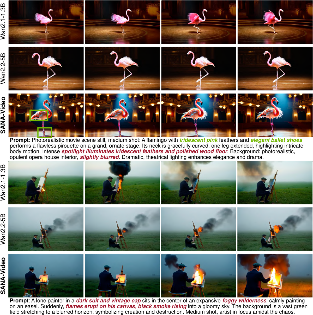
Figure 6 解读: T2V qualitative comparison 展示 SANA-Video 在文本语义、主体运动和画面一致性上接近或优于小型 SOTA diffusion models。该图不能替代表格数值，但能补充说明 Semantic=81.35 的来源：SANA-Video 不是只靠低延迟取胜，而是在保持 prompt adherence 的同时降低计算。

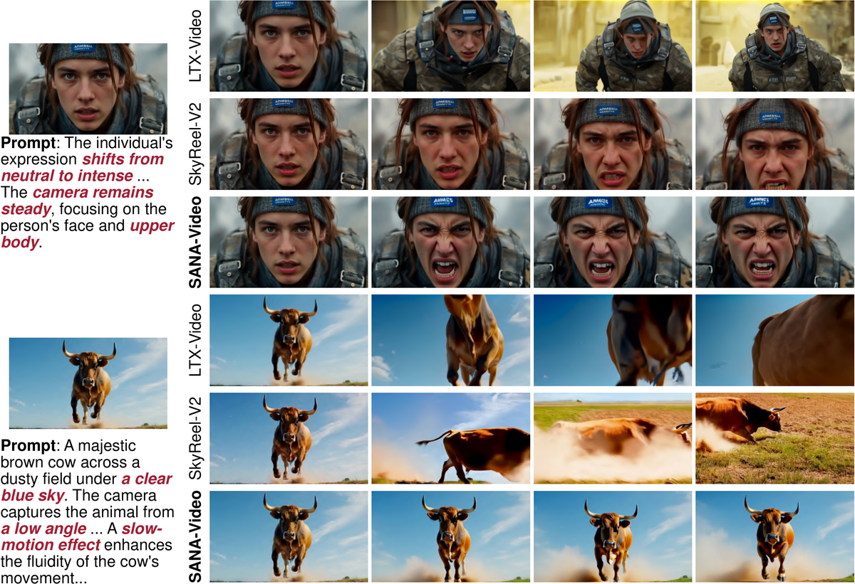
Figure 7 解读: I2V qualitative comparison 强调首帧一致性和 motion control。结合主表 I2V=96.40，可见 SANA-Video 在图像条件保持方面优于多数组合式大模型；这与高质量 captioning、SFT filtering、以及 temporal Mix-FFN 的局部运动建模共同相关。

5.2 720p results and quantization

Model	Latency(s)	Total ↑	Quality ↑	Semantic ↑
Wan-2.1-14B	1897	83.73	85.77	75.58
Wan-2.1-1.3B	400	83.38	85.67	74.22
Wan-2.2-5B	116	83.28	85.03	76.28
SANA-Video-2B	36	84.05	84.63	81.73

720p 设置下，SANA-Video-2B 的 36s latency 是表内最低，同时 Total=84.05 与 Semantic=81.73 最高。论文还报告 RTX 5090 上 NVFP4 precision 可以把 5s 720p video 的 generation latency 从 71s 降到 29s，约 2.4× speedup。这说明部署优化并不是只在 H100 上成立；NVFP4 量化后，edge / prosumer GPU 也进入可用区间。

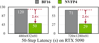
Figure 8 解读: Quantization 图对比 BF16 与 NVFP4 latency。重点不是量化本身的新颖性，而是 Linear DiT 的计算结构足够规则，能和低精度 kernel 叠加加速；如果 backbone 仍是 heavy full attention，NVFP4 只能部分缓解矩阵乘成本，无法解决长序列 cache 与 attention map 的瓶颈。

5.3 Ablations: 3D RoPE, temporal Conv, linear attention, SNR sampler

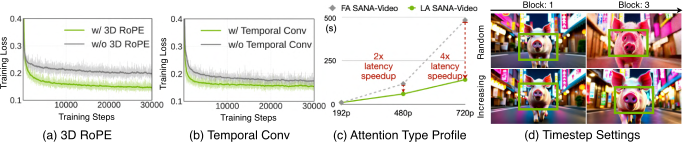
Figure 9 解读: Ablation 图包含四个关键实验：(a) 去掉 3D RoPE 后 training loss 更高，说明 video token 不能只靠 content kernel 聚合，仍需要显式时空位置；(b) 去掉 temporal 2D/1D convolution 后 loss 上升，说明 Mix-FFN 的局部时序归纳偏置是 linear attention 的补偿项；(c) linear attention 相比 full attention 在 latency 上更优；(d) LongSANA 的 monotonically increasing SNR sampler 比 random timestep sampling 在跨 block consistency 上更稳定。

这些 ablation 支持一个重要结论：SANA-Video 的效率不是单点 trick。Linear attention 降低 attention 主项，3D RoPE 保留位置感，temporal convolution 弥补局部 motion modeling，monotonic SNR sampler 则让 autoregressive block training 更接近推理时的噪声递进。任一组件缺失都会让“快但稳定”的目标变弱。

5.4 Constant-memory attention and long video generation

Metric	Causal Full Attention	Causal Local Attention	Causal Linear Attention
Memory	$O (N \times D)$	$O (W \times D)$	$O (D^{2})$
Compute cost for N-th token	$O (N \times D)$	$O (W \times D)$	$O (D^{2})$
Compute cost for N tokens	$O (N^{2} \times D)$	$O (N \times W \times D)$	$O (N \times D^{2})$

LongSANA 的关键不是只把短视频拼接起来，而是让每个 block 通过 causal linear state 读到所有历史。论文表述中，causal linear DiT 保存两类固定状态：attention 侧的 cumulative attention states / cumulative keys，以及 Mix-FFN 侧的 previous block last frame。这样新的 block 不需要把所有旧 frame 的 KV 都放回显存。

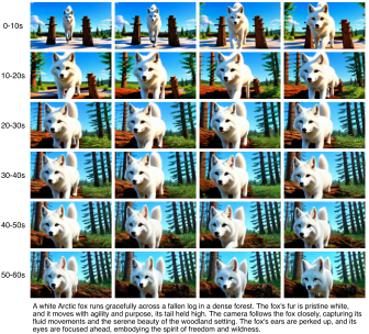
Figure 10 解读: LongSANA visualization 展示 minute-scale 生成的连续性。与 main 5s benchmark 相比，这里更关注跨 block identity、scene layout 与 motion direction 是否持续；constant-memory KV cache 的价值就在于让 block 之间有全局历史，而不是每 5s 重启一次 generation。

论文报告 4-step LongSANA 可以在单 H100 上 35s 生成 1-minute、16FPS、480P video，达到约 27FPS generation speed。这个数字说明 LongSANA 的目标已经接近 real-time generation，但它依赖 4-step setting、480P resolution 与特定 H100 测试条件，不能直接外推到所有 prompts / 所有分辨率。

5.5 Autoencoder and data-quality effects

DCAE-V / high-compression VAE 的结果说明：更高压缩比会牺牲一部分 clean reconstruction 指标，但能显著降低 latent token 的空间尺寸，从而放大 Linear DiT 的效率收益。

Autoencoder	Ratio	PSNR ↑	SSIM ↑	LPIPS ↓
F8T4C16 (Wan2.1-VAE)	16	34.41	0.95	0.01
F16T4C48 (Wan2.2-VAE)	21	35.61	0.96	0.01
F32T8C128 (LTX-VAE)	64	32.26	0.93	0.04
F32T4C32 (DCAE-V)	128	33.25	0.94	0.03

在 clean reconstruction 上，DCAE-V 不如 Wan2.1 / Wan2.2-VAE；但在 $ϵ = 0.1$ 与 $ϵ = 0.2$ 噪声扰动下，DCAE-V 的 PSNR / SSIM / LPIPS 反而更稳： $ϵ = 0.1$ 时 DCAE-V 为 31.91 / 0.93 / 0.04， $ϵ = 0.2$ 时为 29.34 / 0.90 / 0.05。对 diffusion latent denoising 来说，这种 noise robustness 可能比 clean pixel reconstruction 更重要。

Figure 11 解读: SFT 图展示 human-preferred 5,000 条高质量视频 fine-tuning 的影响：细节质量、物理合理性与 motion realism 都会改善。它解释了为什么数据过滤不是附属工程；对于一个小型 2B 模型，训练数据的 motion / aesthetic / saturation 分布直接决定了模型是否能用较低 compute 学到稳定运动。

5.6 局限与实践注意点

质量-效率 trade-off: SANA-Video 在 latency 和 semantic/I2V 上很强，但 480p T2V 的 Quality=84.35 低于 Wan2.1-1.3B 的 85.23 和 Wan2.1-14B 的 85.59；低成本并不表示所有视觉细节都最好。 Autoencoder trade-off: DCAE-V 的 128× compression 带来速度收益，但 clean PSNR / SSIM 低于较低压缩 VAE；实际部署中要根据 resolution、VAE、refiner pipeline 决定是否接受该损失。 Code/docs naming caveat: 论文称 720p 路径为 DCAE-V，公开 docs/config 中还出现 LTX2VAE_diffusers 与 LTX2 Refiner pipeline；复现实验时必须固定 checkpoint、VAE 与 config，不能只按论文名概括。 数据规模未完整公开: 论文说明了 filtering pipeline 和约 5,000 条 SFT videos，但没有完整公开 pre-training clip 总数；因此只能复现 pipeline 思路，不能从论文直接复现完整数据规模。

Paper Notes

探索

SANA-Video: Efficient Video Generation with Block Linear Diffusion Transformer

SANA-Video: Efficient Video Generation with Block Linear Diffusion Transformer

1. Motivation (研究动机)

1.1 视频生成的计算瓶颈

1.2 现有方法的局限

1.3 核心问题

2. Idea (核心思想)

3. Method (方法)

3.1 整体架构

3.2 Linear Attention with RoPE

问题: 将 RoPE 集成到 Linear Attention

解决方案: RoPE(ReLU(x)) 而非 RoPE(x)

3.3 Mix-FFN with Spatial-Temporal Convolution

3.4 Block Linear Attention with Constant-Memory KV Cache

Causal Linear Attention 的 KV Cache 重新推导

Block Causal Mix-FFN

3.5 训练策略

Stage 1: VAE Adaptation (T2I)

Stage 2: Continue Pre-Training from T2I

Stage 3: Autoregressive Block Training (LongSANA)

3.6 Deep Compression Video Autoencoder (DCAE-V)

3.7 Released Code 对照与实现核查

4. Experimental Setup (实验设置)

4.1 模型配置

4.2 Evaluation

4.3 数据与过滤设置

4.4 Baselines 与指标定义

5. Experimental Results (实验结果)

5.1 Main VBench results: 480p / 81 frames

5.2 720p results and quantization

5.3 Ablations: 3D RoPE, temporal Conv, linear attention, SNR sampler

5.4 Constant-memory attention and long video generation

5.5 Autoencoder and data-quality effects

5.6 局限与实践注意点

目录

反向链接