LongLive-2.0: An NVFP4 Parallel Infrastructure for Long Video Generation

Paper: arXiv:2605.18739 Code: NVlabs/LongLive Code reference: main @ 4f53802c (2026-05-18)

1. Motivation (研究动机)

Figure 0 解读：teaser 同时给出 qualitative 与 system-side 结果。左侧对比 BF16 与 NVFP4 生成的五个 shots，强调 NVFP4 没有明显破坏场景构图、主体结构和 shot-level semantics；右侧把训练与推理效率放在一起，给出 2.15× training speedup、1.84× inference speedup、以及 45.7 FPS 的实时推理目标。它也暗示本文的评估重点：不仅要看视频质量，还要看长视频系统在显存和端到端延迟上的可用性。

LongLive-2.0 解决的不是“再提出一个更长的视频生成 loss”这一类单点算法问题，而是长视频生成在训练、推理、量化和交互部署上被系统瓶颈卡住的问题。长视频 AR diffusion 的目标很自然：把视频拆成时间块，当前块在 clean history 的条件下生成，这样可以支持连续续写、prompt 切换和分钟级视频。但一旦把这个目标真正扩展到 60s、甚至更长的视频，训练端会遇到序列长度、VAE latent 准备、loss workload 和显存共同膨胀；推理端会遇到 KV cache 线性增长、VAE 解码延迟、低比特量化与质量不一致、以及非 Blackwell GPU 上无法直接使用 NVFP4 Tensor Core 的问题。

论文的动机是把这些问题作为同一个 end-to-end infrastructure problem 来处理，而不是把训练、推理、量化和交互逻辑拆成互不匹配的补丁。已有长视频生成方法多把主要精力放在算法路径上，例如 Self-Forcing 系列通过让模型暴露在自身 rollout 分布中缓解 teacher-forcing mismatch，CausVid、Rolling-Forcing、Context-Forcing 等方法继续讨论 causal student、long tuning、KV recache 或 forcing 机制。

它们证明了 AR video generation 是可行方向，但也让 pipeline 变得复杂：有的需要 ODE initialization，有的需要先做短视频 DMD，再加 streaming long tuning，有的在交互多 shot 场景下仍会遇到 prompt 切换与身份保持之间的冲突。LongLive-2.0 的核心判断是：如果训练基础设施足够强，模型可以直接在 long multi-shot video data 上完成 AR fine-tuning；如果推理基础设施足够强，few-step LoRA、NVFP4、KV cache 压缩和 streaming VAE 可以在一个系统里协同起来。

这篇论文值得关注的原因在于它把“长视频生成质量”和“系统可部署性”绑定起来。对研究者而言，Balanced SP 让 clean-history/noisy-target 的 teacher-forcing layout 可以在 sequence parallelism 下保持目标一致，而不是牺牲 mask 语义换取并行；NVFP4 training 让低比特训练和低比特推理处在一致的数值域里，避免只在部署时做 PTQ；Multi-shot Attention Sink 让多 shot 交互推理在有限 KV window 下仍能同时保存全局身份和当前 shot 的局部连贯性。

对工程部署而言，论文报告 5B 720p 模型在 GB200 上达到 45.7 FPS，同时还能在 H100 等非 Blackwell 平台上用 SP inference 与 4-bit KV cache 降低通信负担。这意味着它的贡献不只是某个 benchmark 分数，而是提供了一条“从长视频训练到实时交互推理”的系统路径。

在当前 vault 的语境里，它和 DMD - One-step Diffusion with Distribution Matching Distillation、CausVid - From Slow Bidirectional to Fast Autoregressive Video Diffusion Models、SANA-Video - Efficient Video Generation with Block Linear Diffusion Transformer 这些工作相邻，但主贡献应归到加速与基础设施：LongLive-2.0 不是单纯追求更好的 temporal consistency，也不是只提出一个新 attention pattern，而是在 NVFP4、SP、KV cache、VAE decode、DMD LoRA 和 multi-shot prompting 之间做 co-design。

2. Idea (核心思想)

核心思想可以概括为：用 chunk-aligned 的并行布局把长视频 AR 训练变成可扩展的 teacher-forcing 任务，再用 NVFP4 把训练和推理的低精度路径打通，最后用多层 KV anchor 与异步 VAE 把模型变成实际可交互的实时长视频系统。与传统“先得到一个模型，再另外做推理加速”的路线不同，LongLive-2.0 从一开始就把训练 layout、低精度数值格式、few-step distillation、cache 策略和 VAE decode 作为同一个 pipeline 设计。第一层创新是 Balanced SP。

普通 sequence parallelism 会按 token 维度切分序列，但 AR teacher forcing 的序列不是普通序列：它由 clean history stream 和 noisy target stream 拼接而成，loss 只落在 noisy target 上。如果粗暴切分 [all clean; all noisy]，某些 rank 会 clean-heavy，某些 rank 会 noisy-heavy，loss 和 backward workload 不均衡，而且 VAE 编码仍可能在每个 rank 上重复。

Balanced SP 改成让每个 rank 拥有同一时间范围的 clean chunk 与 noisy chunk，即 $z^{(p)} = [z_{c l e an}^{(p)}, z_{n o i sy}^{(p)}] \in R^{L / P \times H \times d}$ 。这样每个 rank 同时有上下文和监督目标，VAE 也只需要编码局部 raw-video chunk 加 halo。第二层创新是 NVFP4 end-to-end。

论文不是只在 inference 做 PTQ，而是在 AR training、DMD LoRA distillation、W4A4 inference 和 KV cache quantization 中都显式使用 NVFP4。NVFP4 用 E2M1 FP4 值、16-element FP8 E4M3 block scale 和 FP32 tensor-level global scale 表示张量： $\hat{X} = \hat{X}^{FP 4} \cdot α^{FP 8} \cdot α^{FP 32}$ 。这个格式在 Blackwell GPU 上有硬件支持，能让 linear/GEMM-heavy 的 long-video DiT 直接受益。

作者还把 LoRA 写成 $W ≃ De q u an t (Q (W_{0})) + Δ W$ ，保留 backbone 的量化权重，同时让少量 LoRA 参数承接 DMD few-step 能力。

第三层创新是 inference 的交互化设计。普通 attention sink 只固定视频开头，适合保留全局身份，但多 shot 场景中 prompt 变化会造成新 shot 局部一致性不足；如果只移动当前 shot sink，又容易丢全局身份。Multi-shot Attention Sink 同时维护 global sink $A_{g}$ 和 shot-level sink $A_{s}$ ，有效 KV 集合是 $K_{e ff} (t) = A_{g} \cup A_{s} \cup K V_{[t - W, t)}$ 。

prompt switch 被当成 scene cut，触发 $A_{s}$ re-bind，而 $A_{g}$ 和历史 cache 保持不动。这个机制把“用户切换 prompt”的语义直接映射到 KV cache 的 anchor 更新规则。

与 Self-Forcing 系列相比，LongLive-2.0 的根本区别不是“再训练一个 AR 模型”，而是把基础设施提升到足够强后，减少算法 pipeline 的阶段数：直接从 Wan2.2-TI2V-5B 做 long multi-shot AR fine-tuning，再用 standalone LoRA 从 4-step 转到 2-step/real-time，而不是依赖 ODE init、短视频 DMD、streaming long tuning DMD 的多阶段堆叠。它的代价是对硬件和实现路径更敏感：NVFP4 加速主要依赖 Blackwell；非 Blackwell 需要通过 SP inference 与 4-bit KV cache 通信压缩来弥补。

3. Method (方法)

3.1 总体框架：训练 infra、推理 infra、算法 clean pipeline 三层耦合

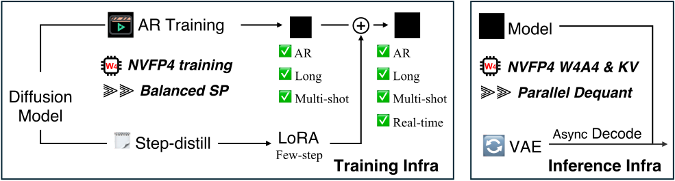
Figure 1 解读：左侧是 training infra，核心是 long-video AR fine-tuning + Balanced SP + NVFP4；右侧是 inference infra，核心是 W4A4 NVFP4 generator、NVFP4 KV cache、以及异步 VAE decode。图中最重要的关系是：DMD LoRA 不再是一个独立大模型分支，而是从 AR generator 旁路训练出 standalone weights，在推理时注入或合并，使同一个 long-video AR backbone 获得 few-step 能力。换言之，LongLive-2.0 把“训练得起长视频”和“推理跑得动长视频”放在同一张图里，而不是先做质量再单独压缩。

整体 pipeline 有三个阶段。第一，使用 Wan2.2-TI2V-5B 作为 base model，冻结 text encoder 与 VAE，把 bidirectional diffusion model 直接 fine-tune 成 long、interactive、multi-shot 的 AR diffusion model。第二，在 AR 模型基础上做 DMD LoRA distillation：backbone 冻结，只训练 LoRA adapter，得到可以让 4-step 甚至 2-step 推理工作的 standalone LoRA。第三，在部署时组合 NVFP4 W4A4 inference、KV cache quantization、multi-shot attention sink 和 streaming/asynchronous VAE decoding，目标指标不只是 DiT-only FPS，而是 end-to-end generation latency/FPS。

直觉上，这个框架成功的关键是各层接口保持一致。Balanced SP 让训练时每个 rank 看到 clean/noisy 对齐的 temporal chunk；multi-shot prompting 让每个 chunk 绑定自己的文本条件；inference 端的 scene cut 与 shot-level sink 也按 chunk 更新。这样训练时的 chunk-level AR 语义、推理时的 KV cache 更新语义、以及用户交互时的 prompt 切换语义都落在同一个 temporal unit 上。若没有这一点，即使某个部分单独很快，也容易出现训练目标、prompt 控制和缓存机制互相打架。

3.2 Balanced SP：把 teacher-forcing AR layout 改造成并行友好的 chunk layout

Figure intuition：balanced vs traditional SP

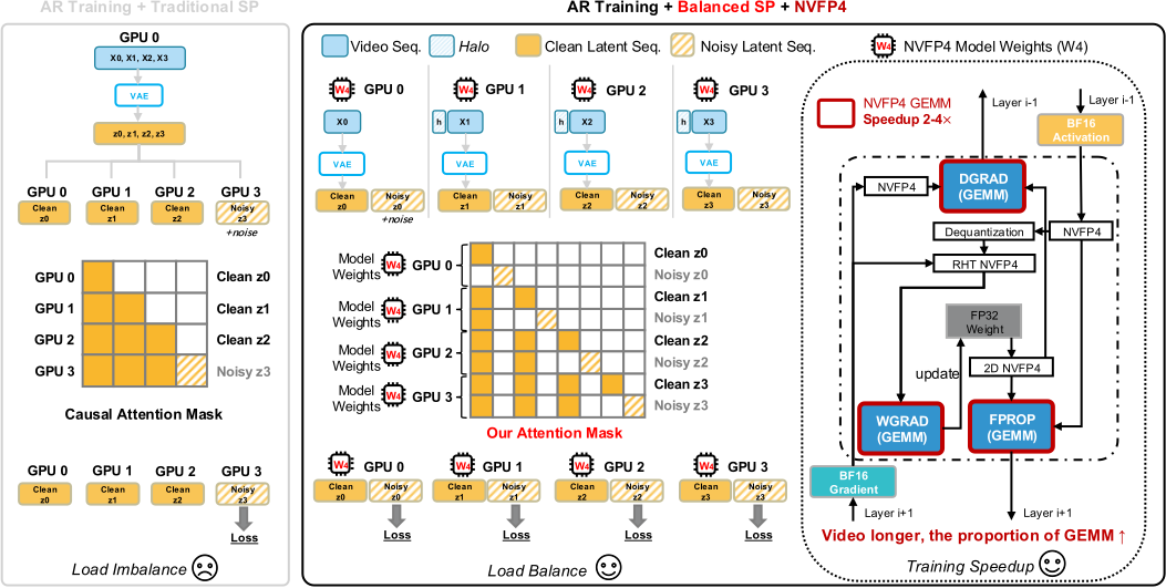
Figure 2 解读：左侧的 Traditional SP 把 clean history 和 noisy target 拼成普通长序列后切分，这会导致 clean-heavy/noisy-heavy 的 rank 分布；loss-bearing token 不均衡，并且 VAE latent preparation 仍可能复制。中间的 Balanced SP 用相同 temporal ownership 管理 clean stream、noisy stream、SP attention、VAE encoding 和 loss computation；右侧的 NVFP4 与 Balanced SP 正交，用低精度 GEMM 降低 memory traffic 和计算时间。图的核心不是“多用了一个并行策略”，而是把 AR teacher forcing 的语义顺序改写成通信友好的顺序。

Parallel teacher forcing

论文先采用 efficient parallel teacher forcing：给定 $N$ 个 temporal chunks 的 raw video window $X$ ，VAE 编码得到 latent $Z$ ，构造 clean/noisy 双流 $[z_{c l e an}; z_{n o i sy}]$ ，用 block-sparse AR mask 让每个 noisy chunk 可以看之前 clean chunks 和自己的 noisy tokens，因此一个 forward pass 能监督所有 noisy chunks。这个设计避免了逐 suffix 训练的低效，但序列长度翻倍，且 clean/noisy 的结构性很强，不能直接当成普通 token sequence 切。

Paired rank layout

Balanced SP 的布局是：对第 $p$ 个 SP rank，持有同一 temporal range 的 clean 与 noisy latent： $z^{(p)} = [z_{c l e an}^{(p)}, z_{n o i sy}^{(p)}] \in R^{\frac{L}{P} \times H \times d} .$ 这个 paired layout 有两个作用。第一，每个 rank 都包含目标 noisy token，loss workload 更均衡；第二，VAE 编码也按相同 temporal chunk 分片。具体来说，每个 rank 只 VAE-encode 自己的 raw-video chunk $X^{(p)}$ 加一个 left halo，用 halo 覆盖 VAE temporal receptive field，编码后丢弃 halo latent，只保留精确的本地 latent chunk $Z^{(p)}$ 。若 latent frame 数是 $F$ ，halo 大小是 $h$ ，原本每 rank 重复 VAE 的成本是 $O (F)$ ，Balanced SP 降为 $O (F / P + h)$ 。

Communication order and AR mask

Ulysses All-to-All 之后，paired layout 会自然变成 interleaved global order，而不是传统 [all clean; all noisy]。作者不在每个 attention layer 重新 materialize permutation，而是在通信原生顺序上直接构造 AR mask，并用 flex_attention 编译。这个做法非常重要：它保留 teacher-forcing visibility，又避免为了恢复逻辑顺序而频繁搬运 tensor。

Released code mapping

released code 中 wan_5b/distributed/sp_training.py 的 SequenceParallelHelper.partition_training_inputs 负责对 clean latent 与 conditional dict 分片，build_loss_mask 与 partition_loss_mask 处理局部/全局有效 token 计数，encode_raw_video_latents 依赖 sp_vae_chunk_meta 完成 chunk-halo VAE 编码；

trainer/diffusion.py::Trainer.train_one_step 在 raw video 时先调用 helper 编码，再构造 loss mask，最后把分片后的输入交给 model.generator_loss。

Balanced SP 伪代码（对应 `trainer/diffusion.py` 与 `wan_5b/distributed/sp_training.py`）

def balanced_sp_train_step(batch, model, sp_helper, optimizer, accum_steps):
    if batch["raw_video"] is not None:
        clean_latent, image_latent, is_sharded = sp_helper.encode_raw_video_latents(
            batch, batch_size=batch["raw_video"].shape[0]
        )
    else:
        clean_latent = batch["ode_latent"][:, -1].cuda()
        image_latent = clean_latent[:, :1]
        is_sharded = False
 
    loss_mask = sp_helper.build_loss_mask(batch, clean_latent, is_sharded)
    cond = model.text_encoder(batch["prompts"])
 
    if sp_helper.enabled():
        clean_latent, cond, latent_shape = sp_helper.partition_training_inputs(
            image_or_video_shape=list(clean_latent.shape),
            clean_latent=clean_latent,
            conditional_dict=cond,
            clean_latent_is_sharded=is_sharded,
        )
    else:
        latent_shape = list(clean_latent.shape)
 
    loss_mask, global_valid = sp_helper.partition_loss_mask(
        loss_mask, already_sharded=is_sharded
    )
    loss, logs = model.generator_loss(
        image_or_video_shape=latent_shape,
        conditional_dict=cond,
        clean_latent=clean_latent,
        initial_latent=image_latent,
        loss_mask=loss_mask,
        loss_mask_global_valid_count=global_valid,
    )
    (loss / accum_steps).backward()
    optimizer.step()
    return logs

3.3 AR diffusion loss 与 error recycling：干净上下文不等于忽略 exposure bias

LongLive-2.0 的 AR objective 使用 clean-context teacher forcing，而不是 diffusion forcing。

训练时 model/diffusion.py::CausalDiffusion.generator_loss 对 clean latent 采样 noise 与 timestep，构造 noisy latents 和 flow training target，然后把 clean_x=clean_latent_aug 传给 generator（当 teacher_forcing=true），最后对 flow_pred 与 training_target 做 MSE，并用 loss mask 和 SP 全局有效 token 数归一化。

这个实现与论文的“clean-history/noisy-target”描述一致：模型学习当前 noisy chunk 在 clean generated history 条件下的去噪，而不是只看单个全局 prompt。但论文也承认 pure teacher forcing 仍有残余 exposure bias：训练时 clean prefix 来自 ground truth，推理时 prefix 来自模型自己的 rollout。

released config configs/nvfp4/train_ar_nvfp4.yaml 中开启了 error_recycling：num_buckets=50、buffer_size_per_bucket=500、buffer_warmup_iter=50、context_inject_prob=0.9、latent_inject_prob=0.9、noise_inject_prob=0.01、clean_prob=0.2、clean_buffer_update_prob=0.1、modulate_factor=0.3。

在 code 中，CausalDiffusion.generator_loss 会在 latent/noise/context 三处随机注入 buffer 里的误差，训练 target 仍指向原始 clean latent。这让模型在保持 clean-context teacher forcing 形式的同时，看到一部分接近 rollout error 的上下文。SP-aware error recycling 的细节也很关键。因为 Balanced SP 已经把位置维度按 rank 分片，如果把误差 buffer 全局混用，一个 rank 可能重放另一个 rank 的位置误差，破坏局部可达性。

论文 Appendix C 说明它按 local block position 和 diffusion timestep 做二维 bucket；position 维度被 SP rank 分片，warm-up 时只在相同 SP rank 的 data-parallel ranks 之间 gather buffer entries。这样 checkpoint 也可以每个 SP rank 保存一份，避免 resume 时位置 bucket 错位。

AR loss 与 error recycling 伪代码（对应 model/diffusion.py）：

def causal_diffusion_generator_loss(clean_latent, cond, loss_mask, global_valid=None):
    b, f = clean_latent.shape[:2]
    noise = torch.randn_like(clean_latent)
    timestep_index = sample_blockwise_timestep(f, num_frame_per_block=8)
    timestep = scheduler.timesteps[timestep_index].to(clean_latent.device)
 
    noise_for_train = maybe_inject_noise_error(noise, timestep_index)
    clean_for_noise = maybe_inject_latent_error(clean_latent, timestep_index)
    noisy_latent = scheduler.add_noise(
        clean_for_noise.flatten(0, 1),
        noise_for_train.flatten(0, 1),
        timestep.flatten(0, 1),
    ).unflatten(0, (b, f))
    target = scheduler.training_target(clean_latent, noise_for_train, timestep)
 
    clean_context = maybe_inject_context_error(clean_latent, timestep_index)
    flow_pred, x0_pred = generator(
        noisy_latent,
        conditional_dict=cond,
        timestep=timestep,
        clean_x=clean_context,
        aug_t=None,
    )
    per_token = F.mse_loss(flow_pred.float(), target.float(), reduction="none")
    weighted = per_token * scheduler.training_weight(timestep).unflatten(0, (b, f))
    if loss_mask is not None:
        denom = global_valid if global_valid is not None else loss_mask.sum()
        loss = (weighted * loss_mask).sum() / denom.clamp(min=1.0)
    else:
        loss = weighted.mean()
    update_error_buffers(x0_pred.detach() - clean_latent.detach(), flow_pred.detach() - target.detach())
    return loss

3.4 NVFP4 training 与 DMD LoRA：低比特数值域贯穿训练和推理

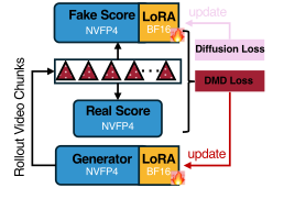
Figure 4 解读：这张图强调 DMD training 不是只量化 generator。DMD 需要 generator、real-score model 和 fake-score model 同时驻留，显存压力比普通 generator fine-tuning 更高。LongLive-2.0 的方案是 progressive NVFP4 conversion：generator 可以是 NVFP4+LoRA，real-score 可以 NVFP4，fake-score 也可以 NVFP4+LoRA，从而把三模型并置的 peak memory 从 BF16 baseline 的 70.5 GB 降到 49.0 GB。

NVFP4 的表示为 E2M1 FP4 值、FP8 E4M3 block scale 与 FP32 global scale。论文中 $B_{i}$ 是第 $i$ 个 16-element block， $M^{FP 8} = 448$ 是 E4M3 最大幅值， $M^{FP 4} = 6$ 是 E2M1 最大幅值。训练时对 linear layers 使用权重 2D block scaling，activation/gradient 1D block scaling；reduction、normalization statistics、optimizer states 保持更高精度。对于梯度敏感路径，论文还使用 RHT 等稳定化技巧。

code 中 utils/quant.py::LongLiveQuantizationConfig 记录 scale rules，utils/nvfp4_kernel.py 提供 fake quant/dequant kernel，utils/nvfp4_checkpoint.py 处理 FourOverSix / Transformer Engine 的 NVFP4 checkpoint materialization。DMD LoRA 的算法接口比原 LongLive 更干净。AR 模型已经支持长视频，因此不需要 ODE initialization、short-video DMD、streaming long-tuning DMD 这样的多阶段堆叠。

LongLive-2.0 在 AR-trained model 上直接做 one-stage DMD distillation，并且不 full fine-tune DiT backbone，而只训练 LoRA。teacher 是原始 Wan2.2-TI2V-5B，student/fake-score/critic 从 AR multi-step DiT 初始化；为了提供 AR supervision，teacher 在 distillation 时也加 causal AR mask。NVFP4 + LoRA 权重路径伪代码（对应 configs/nvfp4/train_dmd_nvfp4_step4.yaml 与 utils/quant.py）：

class QuantizedLoRALinear(nn.Module):
    def __init__(self, fp32_weight, rank=128, alpha=128):
        super().__init__()
        self.q_weight = quantize_to_fp4(fp32_weight, scale_rule="mse")
        self.lora_A = nn.Parameter(torch.empty(rank, fp32_weight.shape[1], dtype=torch.bfloat16))
        self.lora_B = nn.Parameter(torch.empty(fp32_weight.shape[0], rank, dtype=torch.bfloat16))
        self.scale = alpha / rank
 
    def forward(self, x):
        base = F.linear(x, dequantize_fp4(self.q_weight))
        delta = F.linear(F.linear(x, self.lora_A), self.lora_B) * self.scale
        return base + delta

DMD LoRA 伪代码（对应 model/dmd.py）：

def dmd_lora_generator_step(generator, real_score, fake_score, batch):
    generated_x, grad_mask, t_from, t_to = generator.run_generator(
        conditional_dict=batch["cond"],
        initial_latent=batch.get("initial_latent"),
        image_or_video_shape=batch["shape"],
    )
    score_t = sample_score_timestep(min_timestep=0, max_timestep=1000)
    fake_x0 = fake_score(generated_x, timestep=score_t, conditional_dict=batch["cond"])
    real_cond = real_score(generated_x, timestep=score_t, conditional_dict=batch["cond"])
    real_uncond = real_score(generated_x, timestep=score_t, conditional_dict=batch["uncond"])
    real_x0 = real_cond + (real_cond - real_uncond) * 3.0
    grad = (fake_x0 - real_x0).detach()
    target = (generated_x - grad).detach()
    loss = 0.5 * F.mse_loss(generated_x.double(), target.double(), reduction="none")
    return masked_mean(loss, grad_mask)

configs/nvfp4/train_dmd_nvfp4_step4.yaml 中 DMD 的 released 配置是：trainer: score_distillation，distribution_loss: dmd，denoising_step_list: [1000, 946, 854, 681, 0]，real_guidance_scale: 3.0，fake_guidance_scale: 0.0，generator LR 1e-5，critic LR 2e-6，batch size 2，max_iters=5000，dfake_gen_update_ratio=5，num_training_frames=32，LoRA rank/alpha/dropout 在 adapter 中是 128/128/0.0。这些值与 Appendix H 的 DMD 描述基本一致。

3.5 Clean pipeline：基础设施强到可以删除训练阶段

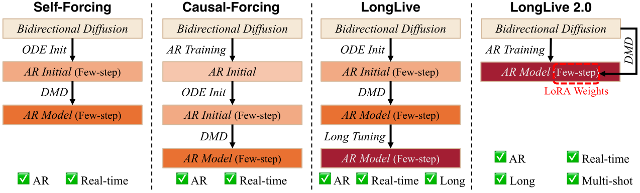
Figure 3 解读：这张图把 LongLive-2.0 与 Self-Forcing / LongLive 类 pipeline 的差别画得很直接。旧路线需要 ODE initialization、短视频 DMD、streaming long tuning 等阶段，才能逐步得到 long、interactive、multi-shot、real-time 能力。LongLive-2.0 先用 long-video data 直接 AR training，再通过 standalone LoRA 注入 few-step 能力，形成更短的两段式流程。图里的“clean”不是说训练目标没有复杂性，而是说复杂性被基础设施吸收了，而不是暴露为多个算法阶段。

这个设计的直觉是：如果 AR training 本身已经可以在长视频上高效运行，那么模型不必先在短序列上学一个代理行为再迁移到长序列；如果 DMD LoRA 可以在量化三模型环境中稳定训练，那么 few-step 能力也不需要绑定到另一个 full fine-tuned backbone。这样做的好处是减少累积误差来源，也让实际部署时的模型组件更清晰：一个 AR generator checkpoint，加一组 LoRA weights，再按硬件选择 NVFP4 inference 或 SP inference。

3.6 Inference infrastructure：W4A4、KV cache、异步 VAE

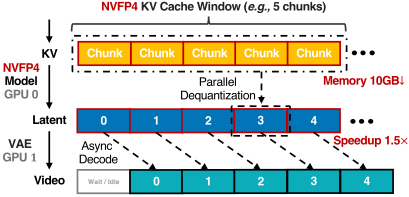
Figure 5 解读：推理图把三个瓶颈串起来：W4A4 NVFP4 降低 DiT 线性层/GEMM 的 memory traffic；KV cache quantization 降低长历史缓存的显存；异步 streaming VAE decode 把最终解码从主 denoising 路径里隐藏掉。注意表格中的 end-to-end FPS 并不只计算 model forward，因此更接近实际用户等待时间。

部署时 generator 以 W4A4 NVFP4 执行，可以是量化 backbone + separate LoRA branch，也可以是 merged W4A4+LoRA 模型。论文指出 AR long-video generation 大量时间在重复 linear layers 和 attention GEMMs 上，FP4 GEMM 理想吞吐可达 BF16 的 4 倍；同时 materialize quantized weights 并 drop BF16 master weights 后，resident memory 也下降。

与 PTQ 不同，它的 backbone 已经经过 NVFP4-aware training，因此 W4A4 inference 的质量损失更小。KV cache 方面，每个 chunk 含 $F_{c} = 8$ frames， $T_{c} = F_{c} L_{f}$ latent tokens；第 $ℓ$ 层第 $c$ 个 chunk 的 cache 是 $K_{ℓ, c}, V_{ℓ, c} \in R^{T_{c} \times H \times d}$ 。KV cache 按 frame-chunk quantize，并使用 k_smooth 之类的处理减少 K 的异常值影响。

released code 中 pipeline/causal_diffusion_inference.py 在 __init__ 读取 kv_quant、kv_quant_scale_rule、kv_quant_backend，构造 LongLiveQuantizationConfig；_initialize_kv_cache 在 quantize_kv 为 true 时以 FP4 quantized tensor 与 zero block 初始化 cache；utils/quant.py::quantize_kv 对每个 head 的 K/V 调用 quantize_to_fp4。

异步 VAE 的想法是把 VAE 解码从“所有 latent 生成完后一次性顺序解码”改成 chunk-by-chunk streaming decode。若共有 $C$ 个 chunks，baseline VAE memory 是 $O (C \cdot T_{c})$ ；streaming decode 降到 $O (T_{c})$ ，并把一个 GPU 专门用于 VAE decode。当 DiT cluster 生成 chunk $c + 1$ 时，VAE GPU 解码 chunk $c$ ；如果 $t_{D i T} \geq t_{V A E}$ ，总延迟从 $C (t_{D i T} + t_{V A E})$ 近似降到 $C \cdot t_{D i T} + t_{V A E}$ 。

code 中 CausalDiffusionInferencePipeline._inference_inner 在 streaming_decode 和 async_vae 打开时把 chunk 放入 queue，由 VAE thread 调 cached_decode 后 offload。

推理路径伪代码（对应 pipeline/causal_diffusion_inference.py）：

def longlive2_inference(noise, text_prompts, generator, vae, cfg):
    kv_pos, kv_neg = initialize_kv_cache(
        batch_size=noise.shape[0],
        dtype=torch.bfloat16,
        quantize_kv=cfg.kv_quant,
        scale_rule=cfg.kv_quant_scale_rule,
    )
    cross_cache = initialize_cross_attention_cache(text_prompts)
    global_sink = cfg.sink_size if cfg.multi_shot_sink else 0
 
    video_chunks = []
    for chunk_index, prompt in enumerate(text_prompts):
        if is_scene_cut(text_prompts, chunk_index):
            pin_current_chunk_as_shot_sink(kv_pos, sink_size=cfg.sink_size)
            reset_cross_attention_cache(cross_cache)
 
        latents = sample_chunk_with_cached_kv(
            generator=generator,
            kv_cache=kv_pos,
            crossattn_cache=cross_cache,
            local_window=cfg.local_attn_size,
            global_sink=global_sink,
            shot_sink_pointer=get_pinned_region(kv_pos),
            sampling_steps=cfg.sampling_steps,
        )
        if cfg.streaming_vae:
            enqueue_or_decode_chunk(vae, latents, async_mode=cfg.async_vae)
        else:
            video_chunks.append(latents)
    return collect_decoded_chunks(video_chunks)

3.7 Multi-shot Attention Sink：全局身份与当前 shot 连贯性分离

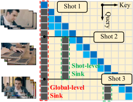
Figure 6 解读：普通 sliding-window attention 只保留近邻 KV，长视频会出现身份和背景漂移；普通 global attention sink 固定最初几帧，可以保全局身份，但多 shot prompt 切换后，当前 shot 的局部动作/场景可能不稳定。LongLive-2.0 把 sink 拆成 global sink 与 shot-level sink：前者永久指向视频开头，后者在 scene cut 后绑定到当前 shot 开头。图中 prompt switch 不需要重算历史，只更新 shot sink pointer 和 cross-attention cache。

有效 KV 集合是： $K_{eff} (t) = A_{g} \cup A_{s} \cup KV_{[t - W, t)} .$ 其中 $A_{g}$ 是前 $S_{g}$ frames，保存角色身份、全局风格和世界状态； $A_{s}$ 是当前 shot 的前 $S_{s}$ frames，在每个 scene cut 重新绑定，保存当前镜头的局部视觉连贯性。released code 的实现非常工程化：_is_scene_cut 由 prompt 是否带 scene cut prefix 与 multi_shot_sink 决定；_pin_current_chunk 不复制数据，只把 pinned_start 和 pinned_len 写进每个 block cache；当窗口滚动后，attention layer 虚拟地把 pinned region prepend 到 sliding window。这个“两个标量 pointer”实现了论文所说的 zero memory overhead。

3.8 非 Blackwell 推理：SP inference 与低比特通信

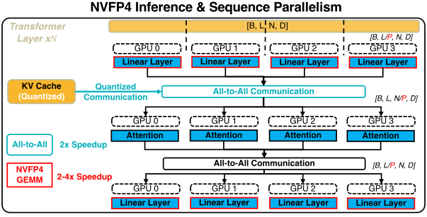
Figure 8 解读：Blackwell 上可以直接从 NVFP4 Tensor Core 得到 W4A4 加速；非 Blackwell（如 H100）缺少同样硬件路径，因此论文把训练用的 Ulysses/SP 思路迁移到 inference。SP 把长序列分摊到多 GPU，但 All-to-All 会引入通信瓶颈；如果 K/V 已在 KV cache 中量化为低比特，SP 交换的 payload 可从 BF16 的 16 bit 降到约 4.5 bit（含 scale overhead），论文报告经验通信量约降 3.6 倍。

released code 中 pipeline/causal_diffusion_inference_sp.py、inference_sp.py 与 wan_5b/distributed/sp_ulysses_inference.py 负责 SP inference；configs/inference_sp.yaml 的关键项是 sp_size: 4、dp_size: 1、model_num_heads: 24、sampling_steps: 4、multi_shot_sink: true、multi_shot_rope_offset: 8、LoRA rank/alpha/dropout 128/128/0.0。这条路径是给非 Blackwell 或超长视频显存受限场景的补偿路线，不等价于 GB200 上的原生 NVFP4 W4A4。

3.9 Figure-level ablations 与 PTQ 对比

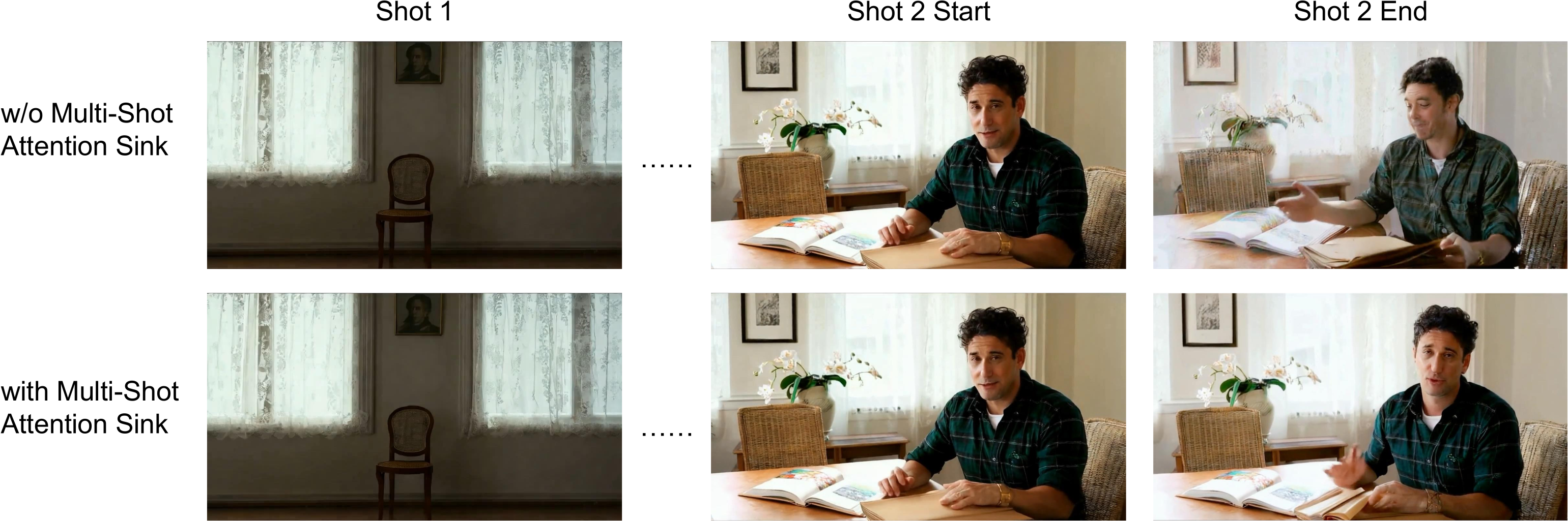
Figure 9 解读：这张 appendix 图是 multi-shot sink 的视觉证据。没有 shot-level sink 时，局部 shot 的主体或背景容易随着窗口滚动发生漂移；只有局部 sink 又可能削弱全局身份。global sink 与 shot sink 同时存在时，模型既能记住整段视频的主体，又能在新 prompt/新 scene 里保持短期连贯性。它支持论文的设计直觉：multi-shot generation 的缓存策略不能只有单一 anchor。

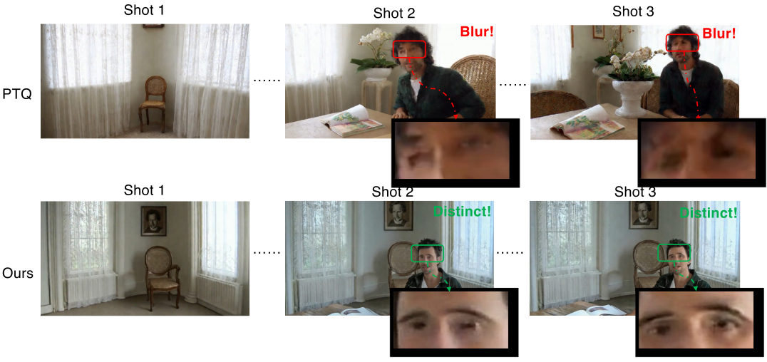
Figure 10 解读：这张图对比 PTQ 与 pre-trained NVFP4。论文的观点是：只在部署时把 BF16 模型 PTQ 到 FP4，质量损失会更明显；如果训练路径已经让模型适应 NVFP4 数值域，W4A4 inference 的语义和画质保留更好。对应 Appendix 表中，BF16 4-step VBench total 是 85.06，NVFP4 PTQ 是 84.04，pre-trained NVFP4 是 84.51，说明预训练/训练时纳入 NVFP4 能追回一部分 PTQ 损失。

3.10 代码锚点与 paper-to-code mapping

论文公式与 released code 实现差异：Appendix H 写 AR training 在 32 张 GB200 上使用 local batch size 1、gradient accumulation 2、global batch size 16，并说默认 AdamW weight decay 是 0.01；但 released configs/nvfp4/train_ar_nvfp4.yaml 中 batch_size: 1、gradient_accumulation_steps: 4、weight_decay: 0.0，如果按 32 GPUs / SP size 4 解读，global batch 会不同。另一个差异是论文 Table 3 展示 + Async Decoding 的推理优化，但 released configs/nvfp4/inference_nvfp4.yaml 默认 streaming_vae: false、async_vae: false；这说明 public config 更像可修改模板，论文实验开关并不全是默认值。下表和伪代码均锚定到当前公开代码 main@4f53802c，训练数值若来自 paper-run 仍以 Appendix H 和论文表格为准。

Code reference: main @ 4f53802c (2026-05-18) — pseudocode and mapping based on this commit

Paper Concept	Source File	Key Class/Function
AR training loop with SP partition	`train.py`, `trainer/diffusion.py`	`Trainer.train`, `Trainer.train_one_step`, `_sync_batch_for_sequence_parallel`
Balanced SP and chunk-halo VAE	`trainer/sp_helper.py`, `wan_5b/distributed/sp_training.py`	`SequenceParallelHelper.encode_raw_video_latents`, `partition_training_inputs`, `partition_loss_mask`
AR flow-matching loss and error recycling	`model/diffusion.py`	`CausalDiffusion.generator_loss`, `_inject_error_buffer`, `_gather_errors_for_buffer`
DMD LoRA distillation	`trainer/distillation.py`, `model/dmd.py`, `configs/nvfp4/train_dmd_nvfp4_step4.yaml`	`Trainer.fwdbwd_one_step`, `DMD.compute_distribution_matching_loss`, `DMD.critic_loss`
NVFP4 model/KV quantization	`utils/quant.py`, `utils/nvfp4_kernel.py`, `utils/nvfp4_checkpoint.py`	`LongLiveQuantizationConfig`, `quantize_to_fp4`, `fp4_dequantize`, `quantize_model_with_filter`
W4A4 inference and async decode	`inference.py`, `pipeline/causal_diffusion_inference.py`, `configs/nvfp4/inference_nvfp4.yaml`	`quantize_generator_model`, `CausalDiffusionInferencePipeline._inference_inner`
Multi-shot attention sink	`pipeline/causal_diffusion_inference.py`	`_is_scene_cut`, `_pin_current_chunk`, `_zero_kv_data`, `_initialize_kv_cache`
SP inference on non-Blackwell GPUs	`inference_sp.py`, `pipeline/causal_diffusion_inference_sp.py`, `wan_5b/distributed/sp_ulysses_inference.py`	`compute_group_specs`, `sp_all_to_all`, `ulysses_seq_to_head`

4. Experimental Setup (实验设置)

4.1 数据集与评测协议

训练数据方面，作者自建了 multi-shot long-video dataset。流程是先把 raw long videos 切成 independent shots，再为每个 shot 标注结构化 caption，覆盖 visual、scene、character、action、cinematography 等维度；之后把同一 full-length video 的 shot captions 合并，并进一步润色成跨 scene temporally coherent 的描述。清洗规则包括去掉过短 shot、logo/watermark/text 明显的视频、严重抖动、异常播放速度、过曝/欠曝、模糊失焦、低运动冻结帧、以及只有轻微 zoom 的片段。视觉质量用 MANIQA 对采样帧评分，最终保留 120K long videos，平均分布在 16–32s、32–64s、over 64s 三个时长组，每组约三分之一。

评测数据与指标分三类。第一，short-video generation 使用 VBench official prompts，并做 prompt augmentation；指标是 VBench Total、Quality、Semantic，另报 throughput FPS、denoising steps、resolution、参数量。第二，long video generation 使用 MovieGenBench prompts 和 VBench-Long；表 5 报 60s generation 的 Avg. Rank、Subject Consistency、Background Consistency、Motion Smoothness、Dynamic Degree、Aesthetic Quality、Imaging Quality。第三，system efficiency 分训练和推理：训练表报告 end-to-end iteration time（seconds）和 speedup；推理表报告 FPS、16/32/64s 的 E2E generation latency 与 peak memory。

4.2 模型、硬件与训练配置

基础模型是 Wan2.2-TI2V-5B。text encoder 和 VAE 全程冻结；默认 BF16 mixed precision、gradient checkpointing、AdamW，论文正文/appendix 说默认 weight decay 0.01，但 released config 有差异，见 §3.10。NVFP4 setting 下，forward、backward、weight-gradient 的 GEMM operands 被量化到 NVFP4，numerically sensitive operations 和 optimizer states 保持高精度。

AR training 的 paper-run 设置是：32 张 NVIDIA GB200，SP size 4，hybrid-full FSDP；每个 SP group local batch size 1，gradient accumulation 2，global batch size 16；训练 600 iterations；generator LR $1.0 \times 1 0^{- 5}$ ，AdamW betas $(0.0, 0.999)$ ；EMA decay 0.99，从 step 100 开始；NVFP4 AR training 消耗 1920 NVIDIA GB200 GPU hours。

released configs/nvfp4/train_ar_nvfp4.yaml 的关键实现设置是：sequence_parallel_size: 4、vae_halo_latents: 28、model_quant: true、model_quant_scale_rule: static_6、model_quant_activation_scale_rule: mse、model_quant_weight_scale_rule: static_6、model_quant_gradient_scale_rule: mse、model_name: Wan2.2-TI2V-5B、num_frame_per_block: 8、sink_size: 8、teacher_forcing: true、num_train_timestep: 1000、denoising_loss_type: flow、max_iters: 600。

DMD LoRA distillation 的 paper-run 设置是：16 张 NVIDIA GB200，local batch size 2，gradient accumulation 1，global batch size 32；训练 5000 iterations；generator LR $1.0 \times 1 0^{- 5}$ ，critic LR $2.0 \times 1 0^{- 6}$ ，AdamW betas $(0.0, 0.999)$ ；critic 每步更新，generator 每五步更新；LoRA rank 128、alpha 128、dropout 0、BF16 adapter weights；

LoRA 作用于 generator 和 fake-score critic 的 causal Wan attention blocks 内 Linear layers；消耗 60 NVIDIA GB200 GPU hours。released configs/nvfp4/train_dmd_nvfp4_step4.yaml 与这些值基本对齐，并且显示 generator 与 real score 都开启 quantization，fake score 在该配置中 fake_score_quant: false，同时对 text embedding、patch embedding、time embedding、norm、head 等模块做 filter。

4.3 推理配置与硬件区分

GB200 / Blackwell 路径使用 NVFP4 W4A4 inference。released configs/nvfp4/inference_nvfp4.yaml 的关键项是：model_name: Wan2.2-TI2V-5B、num_frame_per_block: 8、local_attn_size: 32、sink_size: 8、num_output_frames: 384、latent/image shape [1,384,48,44,80]、sampling_steps: 4、guidance_scale: 1.0、multi_shot_sink: true、multi_shot_rope_offset: 8、kv_quant: true、kv_quant_scale_rule: mse、kv_quant_backend: cuda、model_quant: true、model_quant_use_transformer_engine: true、torch_compile_backend: inductor。注意这个 public config 默认没有开启 streaming/async VAE，论文的 + Async Decoding 结果需要打开相应开关。

非 Blackwell 路径使用 SP inference。configs/inference_sp.yaml 设置 sp_size: 4、dp_size: 1、model_num_heads: 24、sampling_steps: 4、sink_size: 8、multi_shot_sink: true、multi_shot_rope_offset: 8，并加载 generator checkpoint 与 LoRA checkpoint。论文在 H100 上报告 SP=2 和 SP=4 的 latency/communication，说明它是为了没有原生 NVFP4 Tensor Core 加速时降低 per-device memory 与通信 payload。

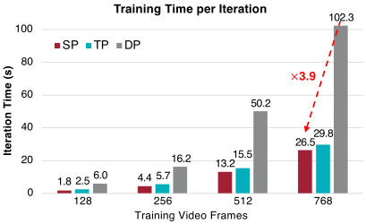
Figure 7a 解读：这张 appendix 子图展示 SP、TP、DP 在 interactive AR video training 上的 iteration speed 随序列长度变化。论文结论是 SP 在被测试长度上最快，且随着上下文变长优势更明显，因为 AR long-video 的瓶颈更接近 sequence length / attention memory，而不是传统模型并行的参数切分。

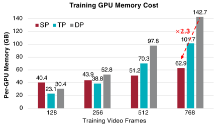
Figure 7b 解读：这张子图补充 peak memory 对比。SP 在长上下文时更省显存，因为每个 rank 持有 sequence shard；而 DP 会复制完整序列，TP 虽能切部分计算但不直接解决长序列缓存和激活膨胀。它为正文选择 Balanced SP 而不是普通 DP/TP 提供了系统证据。

5. Experimental Results (实验结果)

5.1 训练效率：Balanced SP + NVFP4 的收益随长度放大

AR training efficiency 表明，plain BF16 在 16s/32s 上分别是 75.3s/202.7s iteration time，64s OOM；BF16+SP 把 16s/32s 降到 52.2s/162.7s，并让 64s 可运行但仍需 1372.9s；BF16+Balanced SP 进一步降到 45.8s/136.8s/1196.5s；NVFP4+Balanced SP 达到 40.1s/119.3s/639.5s，对 BF16+SP 的 speedup 分别为 1.3×、1.4×、2.1×。最关键的趋势是：视频越长，NVFP4 的 GEMM 加速与 Balanced SP 的 workload/memory 改善越重要；64s 时 NVFP4+Balanced SP 几乎把 BF16+Balanced SP 的时间减半。

DMD NVFP4 scaling 也很直接。三模型全 BF16 时 peak per-GPU memory 是 70.5 GB；generator 改 NVFP4 后为 63.3 GB（0.90×）；generator 用 NVFP4+LoRA、real-score 用 NVFP4、fake-score 仍 BF16 时为 57.2 GB（0.81×）；三者都按最终低精度/LoRA 方案时为 49.0 GB（0.69×）。这相当于每 GPU 减少 21.5 GB，说明 NVFP4 对 DMD 这种多模型同驻场景特别有效。

5.2 推理效率：45.7 FPS 与 64s end-to-end latency 降低

推理表按优化逐步打开。BF16 baseline 是 24.8 FPS，16s/32s/64s 的 E2E latency/memory 为 26.6s/36.4GB、53.2s/36.4GB、112.9s/36.4GB。NVFP4 后 FPS 到 32.0，latency 变成 22.9s/46.6s/96.0s，memory 降到 29.7GB。再加 NVFP4 KV cache 后，FPS 29.7，latency 为 23.8s/48.9s/99.5s，但 memory 降到 19.4GB。再加 Async Decoding 后，FPS 仍 29.7，但 E2E latency 进一步降到 15.9s/29.1s/57.6s。

减少 denoising steps 后，3-step 是 35.2 FPS，16/32/64s latency 为 12.7s/23.2s/46.0s；2-step 是 45.7 FPS，latency 为 11.2s/19.2s/36.3s，memory 保持 19.4GB。这些数字说明三种优化的作用不同：NVFP4 model quantization 主要提升 GEMM throughput；KV cache quantization 主要降显存而不是总是提升 FPS，因为 dequant/scale 也有开销；Async Decoding 主要改善 end-to-end latency，因为它隐藏 VAE decode；

denoising step reduction 则直接减少 DiT loop 次数。论文报告最高 1.84× inference speedup，可以从 BF16 64s latency 112.9s 到 Async 4-step 57.6s 看到接近 2× 的效果，再到 2-step 36.3s 则更快但质量分数进一步下降。在 H100 SP inference 上，单 GPU BF16 的 16s/32s/64s latency 是 31.0s/50.2s/85.0s；SP=2 BF16 降到 19.3s/38.1s/62.5s，通信时间 1.8s/3.2s/5.4s；

SP=2 加 4-bit KV cache 降到 18.3s/36.0s/53.3s，通信时间降到 1.1s/2.3s/3.6s。SP=4 BF16 对 16s 未必更好（26.2s，通信 12.8s），但 4-bit KV cache 后为 21.1s、通信 7.8s；32s/64s 也从 38.6s/65.4s 降到 32.3s/54.8s。结论是 SP 需要低比特通信配合，否则小长度时 All-to-All overhead 会吃掉并行收益。

5.3 VBench 与 VBench-Long：速度提升不是无质量代价，但总体保持强表现

Short-video VBench 表中，LongLive-2.0 BF16 4-step 5B 720p 达到 24.8 FPS，Total/Quality/Semantic 为 85.06/86.67/78.63；NVFP4 4-step 为 29.7 FPS，84.51/86.43/76.81；NVFP4 2-step 为 45.7 FPS，83.14/85.40/74.12。对比 prior LongLive BF16 1.3B 480p 的 20.7 FPS、84.87/86.97/76.47，LongLive-2.0 在更高分辨率和更大模型下保持相近或更高 total，并大幅提升吞吐。

对比 Wan2.2-TI2V-5B BF16 50-step 的 3.3 FPS、83.32/84.95/76.81，LongLive-2.0 的 4-step/2-step 明显更适合实时场景。但质量与速度存在 trade-off。NVFP4 4-step 相对 BF16 4-step 的 Total 从 85.06 降到 84.51，Semantic 从 78.63 降到 76.81；2-step 虽然到 45.7 FPS，但 Total 进一步降到 83.14，Semantic 到 74.12。

论文也特别提醒，VBench 会 resize video 和 sample frames，720p 不一定在 VBench 上比 480p 得分高，因此不能只按分数判断主观质量。更合理的读法是：LongLive-2.0 通过 NVFP4 与 step reduction 提供一条可调的 Pareto curve，用户可以在 4-step 质量和 2-step 实时性之间选择。VBench-Long 60s 表中，LongLive-2.0 BF16 4-step 的 Avg.

Rank 是 3.67，Subject Consistency 97.48，Background Consistency 97.00，Motion Smoothness 98.86，Dynamic Degree 60.62，Aesthetic Quality 53.68，Imaging Quality 65.51；NVFP4 版本 Avg. Rank 3.83，Subject/Background/Motion 为 97.62/96.97/98.94，Dynamic 45.88，Aesthetic 53.72，Imaging 66.24。

它在 Subject、Background、Motion 上非常强，说明 long-context consistency 并没有被低比特或 sliding-window cache 明显破坏；但 Dynamic Degree 在 NVFP4 下下降较多，可能反映低 step / low precision 对运动强度和动作多样性的影响。与 baselines 相比，LongLive-2.0 的 Avg. Rank 好于 LongLive 4.17、Rolling-Forcing 4.50、CausVid 5.33、Self-Forcing 5.83、SkyReels-V2 6.00、Causal-Forcing 6.50、MAGI-1 6.67、NOVA 8.50。

这说明它不是牺牲质量换速度的纯系统优化，而是在长视频一致性指标上也进入第一梯队。LongLive-2.0 NVFP4 的 Avg. Rank 3.83 稍弱于 BF16 3.67，但仍好于旧 LongLive，说明训练时纳入 NVFP4 后，量化部署不会把长视频能力打穿。

5.4 Ablations 与 limitations

NVFP4 precision settings 表明，BF16 4-step 是 Total/Quality/Semantic 85.06/86.67/78.63；NVFP4 PTQ 是 84.04/85.76/77.15；NVFP4 pre-trained 是 84.51/86.43/76.81。pre-trained NVFP4 比 PTQ 的 Total 高 0.47，Quality 高 0.67，但 Semantic 低 0.34；整体支持“训练域适配低精度有帮助”，但不是所有子指标都单调提升。DMD memory ablation 则说明 progressive quantization 对多模型训练显存最有效。

Multi-shot Attention Sink 的视觉 ablation 说明，只有全局 sink 不能同时处理多个 shot 的局部连贯性；只有滑窗容易 drift；global + shot-level sink 能更好地维持全局身份和当前 shot 场景。SP inference table 说明非 Blackwell 场景可用 SP + 4-bit KV cache 补偿，但 SP=4 在短视频时通信 overhead 高，因此不是越大越好。作者明确的 limitation 是硬件依赖。NVFP4 inference 的核心加速依赖 Blackwell GPU（如 GB200）最新 Tensor Cores 和优化 kernel；

A100、H100 没有原生支持，因此只能用 SP inference 等替代路线。另一个实践限制是 public config 与论文实验开关并非完全一致，复现时必须核对 configs/nvfp4/train_ar_nvfp4.yaml、configs/nvfp4/train_dmd_nvfp4_step4.yaml、configs/nvfp4/inference_nvfp4.yaml 和论文 Appendix H，而不能直接把 README 或默认 yaml 当作 paper-run 配置。

5.5 总体结论

LongLive-2.0 的主结论是：长视频生成的质量和速度不能只靠模型结构或 loss 改进解决，必须做训练/推理/数值格式/缓存/解码的全链路 co-design。Balanced SP 让 long AR teacher forcing 在多 GPU 上可训练；NVFP4 让训练和推理共享低比特数值域；DMD LoRA 让 few-step 能力以 adapter 形式注入；Multi-shot Attention Sink 把交互 prompt 切换映射到 KV anchor 更新；Async VAE 把实际用户等待时间降下来。结果上，它在训练端最高 2.1× speedup，推理端最高 1.84× speedup，5B 720p 模型 2-step 达到 45.7 FPS，同时在 VBench 和 VBench-Long 上保持强表现。

从研究价值看，这篇论文最值得复用的不是某一个单独 trick，而是它的接口设计：temporal chunk 是训练并行、prompt binding、KV cache、shot sink 和 VAE decode 的共同单位。只要这个单位稳定，后续可以替换 base model、低比特格式、KV compression 或 attention pruning；如果这个单位不稳定，单独堆加速方法很容易破坏交互控制和长程一致性。因此我会把 LongLive-2.0 归类为 long-video generation infrastructure，而不是普通 video generation algorithm paper。

Paper Notes

探索

LongLive-2.0: An NVFP4 Parallel Infrastructure for Long Video Generation

LongLive-2.0: An NVFP4 Parallel Infrastructure for Long Video Generation

1. Motivation (研究动机)

2. Idea (核心思想)

3. Method (方法)

3.1 总体框架：训练 infra、推理 infra、算法 clean pipeline 三层耦合

3.2 Balanced SP：把 teacher-forcing AR layout 改造成并行友好的 chunk layout

Figure intuition：balanced vs traditional SP

Parallel teacher forcing

Paired rank layout

Communication order and AR mask

Released code mapping

Balanced SP 伪代码（对应 `trainer/diffusion.py` 与 `wan_5b/distributed/sp_training.py`）

3.3 AR diffusion loss 与 error recycling：干净上下文不等于忽略 exposure bias

3.4 NVFP4 training 与 DMD LoRA：低比特数值域贯穿训练和推理

3.5 Clean pipeline：基础设施强到可以删除训练阶段

3.6 Inference infrastructure：W4A4、KV cache、异步 VAE

3.7 Multi-shot Attention Sink：全局身份与当前 shot 连贯性分离

3.8 非 Blackwell 推理：SP inference 与低比特通信

3.9 Figure-level ablations 与 PTQ 对比

3.10 代码锚点与 paper-to-code mapping

4. Experimental Setup (实验设置)

4.1 数据集与评测协议

4.2 模型、硬件与训练配置

4.3 推理配置与硬件区分

5. Experimental Results (实验结果)

5.1 训练效率：Balanced SP + NVFP4 的收益随长度放大

5.2 推理效率：45.7 FPS 与 64s end-to-end latency 降低

5.3 VBench 与 VBench-Long：速度提升不是无质量代价，但总体保持强表现

5.4 Ablations 与 limitations

5.5 总体结论

目录

Paper Notes

探索

LongLive-2.0: An NVFP4 Parallel Infrastructure for Long Video Generation

LongLive-2.0: An NVFP4 Parallel Infrastructure for Long Video Generation

1. Motivation (研究动机)

2. Idea (核心思想)

3. Method (方法)

3.1 总体框架：训练 infra、推理 infra、算法 clean pipeline 三层耦合

3.2 Balanced SP：把 teacher-forcing AR layout 改造成并行友好的 chunk layout

Figure intuition：balanced vs traditional SP

Parallel teacher forcing

Paired rank layout

Communication order and AR mask

Released code mapping

Balanced SP 伪代码（对应 trainer/diffusion.py 与 wan_5b/distributed/sp_training.py）

3.3 AR diffusion loss 与 error recycling：干净上下文不等于忽略 exposure bias

3.4 NVFP4 training 与 DMD LoRA：低比特数值域贯穿训练和推理

3.5 Clean pipeline：基础设施强到可以删除训练阶段

3.6 Inference infrastructure：W4A4、KV cache、异步 VAE

3.7 Multi-shot Attention Sink：全局身份与当前 shot 连贯性分离

3.8 非 Blackwell 推理：SP inference 与低比特通信

3.9 Figure-level ablations 与 PTQ 对比

3.10 代码锚点与 paper-to-code mapping

4. Experimental Setup (实验设置)

4.1 数据集与评测协议

4.2 模型、硬件与训练配置

4.3 推理配置与硬件区分

5. Experimental Results (实验结果)

5.1 训练效率：Balanced SP + NVFP4 的收益随长度放大

5.2 推理效率：45.7 FPS 与 64s end-to-end latency 降低

5.3 VBench 与 VBench-Long：速度提升不是无质量代价，但总体保持强表现

5.4 Ablations 与 limitations

5.5 总体结论

目录

Balanced SP 伪代码（对应 `trainer/diffusion.py` 与 `wan_5b/distributed/sp_training.py`）