Helios: Real Real-Time Long Video Generation Model

Authors: Shenghai Yuan, Yuanyang Yin, Zongjian Li, Xinwei Huang, Xiao Yang, Li Yuan Affiliations: Peking University, ByteDance China, Canva, Chengdu Anu Intelligence

1. Motivation (研究动机)

当前视频生成领域追求实时、长时间、高质量三者兼得，但现有方法都存在根本性局限：

速度瓶颈：主流模型（如 Wan2.1 14B）生成 5 秒视频需约 50 分钟，远达不到实时。即便号称实时的方法也存在问题——Krea-RealTime-14B 在 H100 上仅 6.7 FPS 且漂移严重
小模型困局：现有实时长视频方法（CausVid, Self-Forcing, Rolling Forcing 等）几乎都基于 ~1.3B 小模型，容量不足以建模复杂运动和高频细节
反漂移代价高：Self-Forcing 需要 train-as-infer rollout，Error-Banks 需要额外模块，且它们的鲁棒性与训练时的 rollout 长度强耦合——训练 5 秒片段，推理超过 5 秒就严重漂移
加速技术有副作用：KV-Cache、Causal Masking、Sparse Attention 等改变了双向预训练模型的推理范式，限制了可达质量上限

核心矛盾：大模型质量好但太慢，小模型够快但质量差。

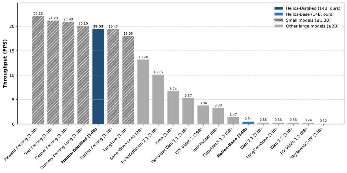
Figure 1 解读：各模型在单卡 H100 上的端到端吞吐量（FPS）对比。深蓝色为 Helios-Distilled（19.53 FPS），浅蓝色为 Helios-Base（0.54 FPS）。斜线填充为 ≤1.3B 小模型，灰色为 ≥2B 大模型。Helios-Distilled 作为 14B 大模型，达到了与 1.3B 小模型蒸馏版（Reward Forcing 22.13、Self Forcing 21.20）相当的速度，远超同尺寸的 Krea（6.74）和 FastVideo（5.37）。

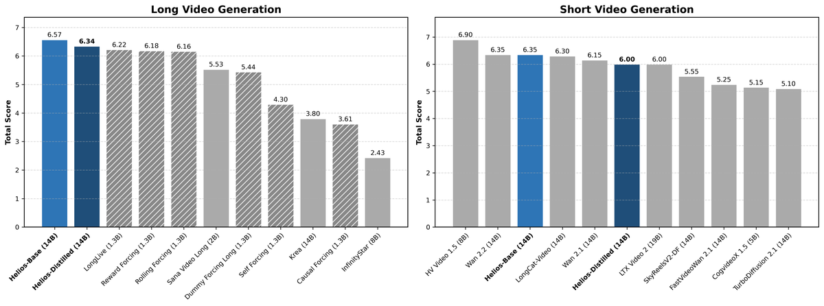
Figure 2 解读：左图为长视频生成的 Total Score，右图为短视频生成的 Total Score。Helios-Base（6.57）和 Helios-Distilled（6.34）在长视频上全面领先；短视频上 Helios-Base（6.35）匹配 Wan 2.1（6.35），Helios-Distilled（6.00）超越所有蒸馏模型。

2. Idea (核心思想)

Helios 的核心 insight：14B 大模型可以比 1.3B 小模型更便宜、更快、同时更强。

实现路径是从三个独立维度同时发力，每个维度都避开了前人的常见陷阱：

Unified History Injection：不用 Causal Masking（破坏双向注意力），而是通过 Representation Control + Guidance Attention 将双向模型改造为自回归生成器
Easy Anti-Drifting：不用 Self-Forcing（训练昂贵 + 长度依赖），而是直接在训练中模拟漂移的三种表现形式（位置/颜色/恢复偏移）
Deep Compression Flow：不用 KV-Cache 或 Sparse Attention，而是从 token 数量（Multi-Term Memory Patchification + Pyramid UniPC）和采样步数（Adversarial Hierarchical Distillation）两个维度深度压缩计算量

最终结果：14B 模型在单卡 H100 上 19.5 FPS，计算量降到与 1.3B 模型可比，质量超越所有同类方法。

3. Method (方法)

3.1 整体架构

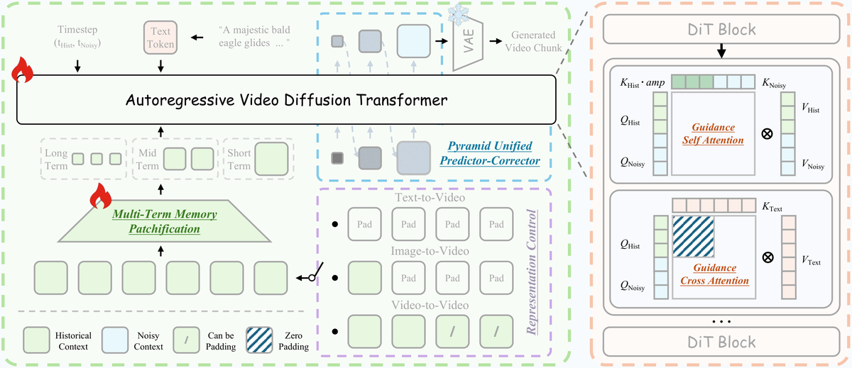
Figure 4 解读：整体架构图。左下方：历史上下文（绿色）和噪声上下文（灰色）拼接为输入，经 Multi-Term Memory Patchification 分层压缩（Long/Mid/Short 三级 Conv3d）。中间：Autoregressive Video Diffusion Transformer 主体。右上方：Guidance Attention 的两种形式——Self-Attention 中历史和噪声 token 共同参与但用 $am p$ 调制历史 key；Cross-Attention 中仅噪声 token 接收文本信息。右侧：Pyramid Unified Predictor Corrector 从低分辨率逐步上采样到全分辨率。底部：Representation Control 通过零填充/帧填充自动切换 T2V/I2V/V2V 任务。

Helios 是一个 14B Autoregressive Video Diffusion Transformer，基于 Wan-2.1-T2V-14B 初始化。核心架构改动：

输入拼接：历史上下文 $X_{Hist}$ （干净，经 Multi-Term Memory Patchification 压缩）+ 噪声上下文 $X_{Noisy}$ （待去噪）
注意力机制：Guidance Self-Attention（区分历史/噪声 token 的角色）+ Guidance Cross-Attention（仅对噪声 token 注入文本语义）
任务统一：通过 $X_{Hist}$ 的内容自动切换 T2V/I2V/V2V

三阶段渐进训练：

Stage 1 (Base)：架构改造（Unified History Injection + Easy Anti-Drifting + Multi-Term Memory Patchification）
Stage 2 (Mid)：token 压缩（引入 Pyramid Unified Predictor Corrector）
Stage 3 (Distilled)：step 蒸馏（Adversarial Hierarchical Distillation，50 步 → 3 步）

3.2 Unified History Injection

Representation Control：将长视频生成建模为视频续写任务。

Input = Concat (X_{Hist} \in R^{B \times C \times T_{Hist} \times H \times W}, X_{Noisy} \in R^{B \times C \times T_{Noisy} \times H \times W})

其中 $T_{Hist} ≫ T_{Noisy}$ 。模型对 $X_{Noisy}$ 去噪，以 $X_{Hist}$ 为条件。任务切换通过 $X_{Hist}$ 内容自动实现：全零 → T2V；仅最后一帧非零 → I2V；多帧非零 → V2V。

Guidance Attention：历史上下文（干净信号）和噪声上下文（待去噪）统计特性不同，必须区别对待。

Self-Attention 中引入 head-wise amplification token $am p$ 来调制历史 key，选择性放大或抑制每个 attention head 中的历史信息：

X_{Self} = Attention ([Q_{Noisy}, Q_{Hist}], [K_{Noisy}, K_{Hist} \cdot am p], [V_{Noisy}, V_{Hist}]) (1)

Cross-Attention 仅作用于 $X_{Noisy}$ （历史帧已包含文本语义，重复注入是冗余的）：

X_{Cross} = Attention (Q_{Noisy}, K_{Text}, V_{Text}) (2)

历史帧的 timestep 固定为 0（表示干净、无噪声），整个去噪过程中不会被修改。

def guidance_attention_block(hidden_states, encoder_hidden_states, amp, navit_mask):
    """Per transformer block: Guidance Self-Attention + Cross-Attention + FFN."""
    # --- Self-Attention with history amplification ---
    Q, K, V = qkv_proj(norm1(hidden_states))
    Q_noisy, Q_hist = split(Q, at=noisy_seq_len)
    K_noisy, K_hist = split(K, at=noisy_seq_len)
    V_noisy, V_hist = split(V, at=noisy_seq_len)
 
    K_hist = K_hist * amp  # head-wise amplification (learnable per-head)
 
    attn_out = flash_attention(
        Q=concat(Q_noisy, Q_hist),
        K=concat(K_noisy, K_hist),
        V=concat(V_noisy, V_hist),
    )
    hidden_states = hidden_states + attn_out
 
    # --- Cross-Attention: only noisy tokens attend to text ---
    noisy_states = hidden_states[:noisy_seq_len]
    Q_noisy = q_proj(norm2(noisy_states))
    K_text, V_text = kv_proj(encoder_hidden_states)
    cross_out = attention(Q_noisy, K_text, V_text, mask=navit_mask)
    hidden_states[:noisy_seq_len] += cross_out
 
    # --- FFN ---
    hidden_states = hidden_states + ffn(norm3(hidden_states))
    return hidden_states

源码参考：helios/modules/transformer_helios.py → HeliosTransformerBlock.forward()，HeliosAttnProcessor 中 scale_key 实现 amp 放大。

3.3 Easy Anti-Drifting

Figure 5 解读：三种典型漂移模式的可视化。(a) Position Shift：画面在长视频中突然跳到不相关的场景（位置编码超出训练分布）。(b) Color Shift：画面整体色调随时间逐渐偏移（霓虹灯场景变暗/变色）。(c-d) Restoration Shift：画面出现类似图像修复的伪影——(c) 加噪感（粗糙颗粒）和 (d) 模糊感（细节丢失），这是因为模型在不完美的自身输出上反复条件化导致的误差累积。

论文系统地总结了长视频生成中的三种典型漂移模式，并针对性地提出简单有效的解决方案：

a) Position Shift → Relative RoPE

绝对 RoPE 的问题：训练在 5 秒（~109 帧）上，生成 1440 帧视频需要用到 index 0:1399，远超训练分布。此外 RoPE 的周期性与 Multi-Head Attention 交互会导致重复运动（repetitive motion）。

解决方案：限制历史的时间索引为 $0 : T_{Hist}$ ，噪声部分为 $T_{Hist} : T_{Hist} + T_{Noisy}$ 。无论生成多长视频，每次去噪窗口的位置编码范围都固定，消除了分布外和周期性问题。

b) Color Shift → First-Frame Anchor

Figure 6 解读：四个子图分别追踪正常视频（蓝色）和漂移视频（红色）的 Saturation、Aesthetic Score、RGB Mean、RGB Std 随时间的变化。正常视频的所有指标保持平稳，而漂移视频在某个时间点后出现突变——Saturation 骤降、Aesthetic 下降、RGB 均值和方差剧烈波动。这说明漂移不是渐进的，而是在某个临界点后突然恶化，且几乎不在生成开头发生（支持 First-Frame Anchor 的设计动机）。

通过跟踪 saturation、aesthetic score 和 RGB 统计量，发现漂移视频的分布会在某个时间点突然偏移，而正常视频保持稳定。并且漂移几乎不在开头发生。

解决方案：训练和推理时始终保留第一帧在 $X_{Hist}$ 中，作为全局视觉锚点，约束后续帧的统计分布。

c) Restoration Shift → Frame-Aware Corrupt

模型训练在干净历史上，推理在自身不完美输出上——train-test mismatch 导致误差累积。

解决方案：训练时对历史帧独立施加随机扰动：

def frame_aware_corrupt(history_latents, p_a, p_b, p_c, p_d,
                        a_range, b_range, c_range):
    """Training-time corruption to simulate imperfect inference history."""
    # Skip frame 0 — it's the first-frame anchor, always kept clean
    for t in range(1, history_latents.shape[2]):
        frame = history_latents[:, :, t, :, :]
        r = torch.rand(1).item()
 
        if r < p_a:  # exposure adjustment
            scale = uniform(a_range[0], a_range[1])  # e.g. [0.3, 1.7]
            frame *= scale
        elif r < p_a + p_b:  # add noise
            sigma = uniform(b_range[0], b_range[1])  # e.g. [0, 0.33]
            frame += torch.randn_like(frame) * sigma
        elif r < p_a + p_b + p_c:  # downsample + upsample (blur)
            ratio = uniform(c_range[0], c_range[1])  # e.g. [0, 0.1]
            frame = F.interpolate(
                F.interpolate(frame, scale_factor=ratio),
                size=frame.shape[-2:])
        else:  # keep clean (probability p_d)
            pass
 
    return history_latents

源码参考：helios/utils/utils_helios_base.py → corrupt_history_latents()，add_saturation_to_history_latents()。实际实现中 is_frame_independent=True 时每帧独立采样 noise sigma。Stage 1 配置： $p_{a} = 0, p_{b} = 0.8, p_{c} = 0.1, p_{d} = 0.1$ ；Stage 3 配置： $p_{a} = 0.4, p_{b} = 0.4, p_{c} = 0, p_{d} = 0.2$ 。

3.4 Deep Compression Flow — Token 维度

Multi-Term Memory Patchification：

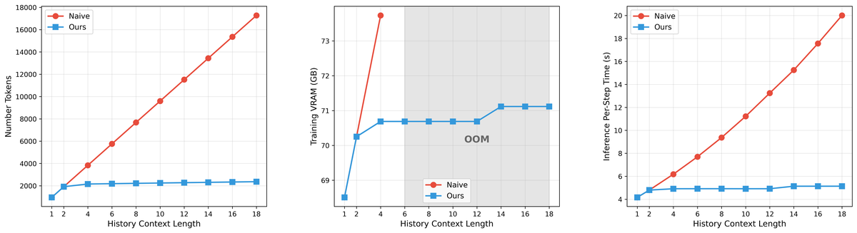
Figure 7 解读：三个子图展示 Multi-Term Memory Patchification 的效果。左图：随着历史长度增加，Naive 方法（蓝色）的 token 数线性增长，而本文方法（红色）保持恒定（约 2000 tokens）。中图：Naive 方法在历史长度 >6 时 OOM，本文方法的训练显存始终稳定在约 71 GB。右图：推理延迟——Naive 方法线性增长，本文方法保持约 5ms 恒定。

核心观察：预测未来帧时，近期历史提供局部运动连续性，远期历史提供粗粒度全局上下文。因此越远的历史可以压缩得越狠。

将 $X_{Hist}$ 分为 short/mid/long 三段（ $T_{1}, T_{2}, T_{3}$ 帧），对每段用不同压缩比的 3D Conv kernel：

L_{total} = H W (\frac{T _{1}}{p _{t}^{(1)} p _{h}^{(1)} p _{w}^{(1)}} + \frac{T _{2}}{p _{t}^{(2)} p _{h}^{(2)} p _{w}^{(2)}} + \frac{T _{3}}{p _{t}^{(3)} p _{h}^{(3)} p _{w}^{(3)}}) (4)

def multi_term_memory_patchify(X_hist, T1=16, T2=2, T3=2):
    """Compress history with increasing patchification for distant frames."""
    # Split into three temporal segments
    hist_short = X_hist[:, :, -T1:, :, :]         # most recent T1 frames
    hist_mid   = X_hist[:, :, -T1-T2:-T1, :, :]   # middle T2 frames
    hist_long  = X_hist[:, :, :-T1-T2, :, :]      # oldest T3 frames
 
    # Apply 3D Conv with increasing compression ratio
    tok_short = patch_short(hist_short)                          # Conv3d(1,2,2) → 4x
    tok_mid   = patch_mid(pad_for_3d_conv(hist_mid, (2,4,4)))   # Conv3d(2,4,4) → 32x
    tok_long  = patch_long(pad_for_3d_conv(hist_long, (4,8,8))) # Conv3d(4,8,8) → 256x
 
    # Flatten spatial dims → (B, num_tokens, D)
    for tok in [tok_short, tok_mid, tok_long]:
        tok = tok.flatten(2).transpose(1, 2)
 
        # Compute per-segment RoPE with relative frame indices
        rope_short = rotary_pos_emb(frame_indices=range(0, T1), H=H1, W=W1)
        rope_mid   = rotary_pos_emb(frame_indices=range(0, T2), H=H2, W=W2)
        rope_long  = rotary_pos_emb(frame_indices=range(0, T3), H=H3, W=W3)
 
        # Concatenate: long (coarse) → mid → short (fine)
        return torch.cat([tok_long, tok_mid, tok_short], dim=1)

实际配置（从源码确认）：

分段	帧数	Conv3d kernel/stride	压缩比	源码定义
Short ( $T_{1} = 16$ )	16	`(1, 2, 2)`	4x	`self.patch_short`
Mid ( $T_{2} = 2$ )	2	`(2, 4, 4)`	32x	`self.patch_mid`
Long ( $T_{3} = 2$ )	2	`(4, 8, 8)`	256x	`self.patch_long`

历史 token 总量减少约 8x，Attention FLOPs 减少约 64x。

源码参考：helios/modules/transformer_helios.py → HeliosTransformer3DModel.__init__() 定义 Conv3d，process_input_hidden_states() 执行拼接和 RoPE。pad_for_3d_conv() 对不整除的帧数做 padding。

Pyramid Unified Predictor Corrector：

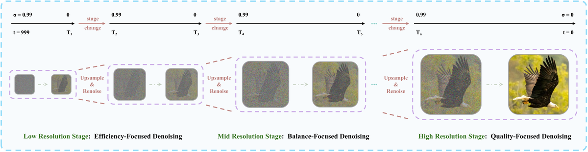
Figure 8 解读：Pyramid Unified Predictor Corrector 的三阶段流程。从左到右：Low Resolution Stage（ $α = 0.99$ ，关注全局布局和颜色）→ Mid Resolution Stage（平衡质量和效率）→ High Resolution Stage（ $α = 0$ ，细化纹理和边缘）。每个阶段结束时通过 Upsample & Renoise 过渡到下一分辨率，并 reset UniPC state buffer 避免跨尺度的 correction 伪影。

对噪声上下文 $X_{Noisy}$ 采用 coarse-to-fine 多分辨率策略。分 $K = 3$ 阶段：低分辨率关注全局结构，高分辨率细化纹理。

每阶段学习从 scale $k - 1$ 到 scale $k$ 的 velocity field：

x_{t}^{k} = (1 - λ_{t}) x^{k} + λ_{t} Up (x^{k - 1}) (5)

L = E [u_{θ}^{k} (x_{t}^{k}, y, λ_{t}, k) - v^{k}_{2}^{2}] (7)

def pyramid_unipc_inference(noise, X_hist, y, K=3):
    """Coarse-to-fine multi-resolution denoising with UniPC solver."""
    x = noise  # starts at lowest resolution: (B, C, T, H/4, W/4)
    boundaries = [1000, T1, T2, 0]  # partition timestep [0, 1000] into K stages
 
    for k in range(1, K + 1):
        timesteps = linspace(boundaries[k-1], boundaries[k], N_k)
        unipc_buffer = UniPCBuffer()  # fresh buffer per stage
 
        for t_prev, t_curr in pairwise(timesteps):
            v = dit(x, X_hist, y, t=t_prev, stage=k)  # predict velocity field
            x = unipc_buffer.update(x, v, t_prev, t_curr)  # multi-step corrector
 
            if k < K:  # transition to next resolution
            x = F.interpolate(x, scale_factor=2, mode='nearest')  # 2x upsample
            x = renoise_correction(x)  # fix distribution shift from upsampling
            unipc_buffer.reset()  # cross-scale predictions are invalid
 
            return x  # full resolution (B, C, T, H, W)

多尺度推理总 token 数相比单尺度减少约 2.29x。

源码参考：helios/scheduler/scheduling_helios.py 管理多阶段 timestep 分配和 UniPC state buffer reset。

3.5 Deep Compression Flow — Step 维度

Adversarial Hierarchical Distillation（基于 DMD 框架）：

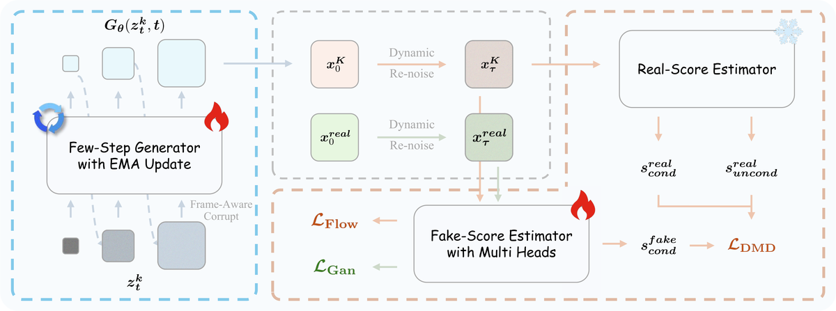
Figure 9 解读：蒸馏 pipeline。左侧：Few-Step Generator（带 EMA 更新）接收噪声 $z_{t}^{k}$ 和历史 $X_{Hist}$ （经 Frame-Aware Corrupt），生成 $x_{0}^{K}$ 。中间上方： $x_{0}^{K}$ 和真实数据 $x_{0}^{real}$ 分别经 Dynamic Re-noise 得到 $x_{τ}^{K}$ 和 $x_{τ}^{real}$ 。右侧：Real-Score Estimator（frozen）输出条件和无条件分数用于 $L_{DMD}$ ；Fake-Score Estimator（trainable）用 $L_{Flow}$ 训练。底部：Multi-head GAN Discriminator 提供 $L_{GAN}$ ，打破对 teacher 分布的依赖。

四项关键改进：

Pure Teacher Forcing：用 Helios-Base 作 teacher（已具备长视频生成能力），配合 Easy Anti-Drifting，仅需每步生成一段即可——不需要 Self-Forcing 的多段 rollout
Staged Backward Simulation：将 backward simulation 分解为 $K$ 阶段独立估计： $x_{0}^{k} = x_{t}^{k} - λ_{t} \cdot u_{θ}^{k} (x_{t}^{k}, y, λ_{t}, k)$
Coarse-to-Fine Learning：(a) Staged ODE Init (b) Dynamic Re-noise（Beta 分布 + cosine 参数调度）
Adversarial Post-Training：在 DiT 的第 5/15/25/35/39 层添加 GAN 判别器头（dim=768）

def adversarial_hierarchical_distillation_step(x_0, y, G_theta, p_real, p_fake, D_heads, step):
    """One training step of Adversarial Hierarchical Distillation (DMD + GAN)."""
    # --- Forward: generate fake sample via staged backward simulation ---
    z_t = torch.randn_like(x_0)
    x_0_staged = G_theta.staged_backward_sim(z_t, y)  # K-stage backward sim
 
    # --- Dynamic Re-noise (Beta distribution with cosine schedule) ---
    tau = Beta(alpha=cosine_schedule(step), beta=cosine_schedule(step)).sample()
    x_tau_fake = add_noise(x_0_staged, tau)
    x_tau_real = add_noise(x_0, tau)
 
    # --- Score estimation ---
    s_real_cond, s_real_uncond = p_real(x_tau_real, y, tau)  # frozen teacher
    s_fake_cond = p_fake(x_tau_fake, y, tau)                  # trainable
 
    # --- DMD loss (distribution matching distillation) ---
    L_DMD = distribution_matching_loss(s_real_cond, s_real_uncond, s_fake_cond)
 
    # --- GAN loss (adversarial post-training) ---
    crop_real = random_crop(x_tau_real, H // 2, W // 2)  # half-res to save memory
    crop_fake = random_crop(x_tau_fake, H // 2, W // 2)
 
    L_D = (torch.log(D_heads(crop_real)).mean()
           - torch.log(D_heads(crop_fake)).mean()
           + 100.0 * approx_r1(D_heads, crop_real, sigma=0.1))  # λ_D=100, σ_D=0.1
    L_G = torch.log(D_heads(crop_fake)).mean()
 
    # --- Flow matching loss (stabilizer for p_fake) ---
    L_Flow = F.mse_loss(p_fake.predict_velocity(x_tau_fake), v_target)
 
    # --- Combined losses ---
    L_generator = L_DMD + 0.05 * L_G    # w_G = 5e-2
    L_estimator = L_Flow + 0.01 * L_D   # w_D = 1e-2
 
    # --- TTUR: update p_fake every step, G_θ every 5 steps ---
    optimizer_fake.zero_grad(); L_estimator.backward(); optimizer_fake.step()
    if step % 5 == 0:
        optimizer_G.zero_grad(); L_generator.backward(); optimizer_G.step()

源码参考：train_helios.py → _generator_loss() 和 _critic_loss()；GAN heads 定义在 transformer_helios.py。实际使用 Sharded EMA（ZeRO-3）+ Async VRAM Freeing + Cache Grad for GAN 来优化显存。

Figure 10 解读：Cache Grad for GAN 的流程示意图，结合前文的 adversarial post-training 设计，说明其通过缓存梯度相关中间量来降低显存占用，并支持判别器头的训练。

3.6 其他推理技术

Adaptive Sampling：用 EMA 跟踪 latent 的全局均值 $\overset{μ}{ˉ}_{t}$ 和方差 $\overset{σ}{ˉ}_{t}^{2}$ ：

\overset{μ}{ˉ}_{t} = ρ_{μ} \overset{μ}{ˉ}_{t - 1} + (1 - ρ_{μ}) μ_{t}, \overset{σ}{ˉ}_{t}^{2} = ρ_{σ} \overset{σ}{ˉ}_{t - 1}^{2} + (1 - ρ_{σ}) σ_{t}^{2}

当偏差超阈值 $∥ μ_{t} - \overset{μ}{ˉ}_{t} ∥_{2} > δ_{μ}$ 或 $∥ σ_{t}^{2} - \overset{σ}{ˉ}_{t}^{2} ∥_{2} > δ_{σ}$ 时，对下一段历史施加 Frame-Aware Corrupt

Interactive Interpolation：用户切换 prompt 时，线性插值 $M$ 步平滑过渡： $e^{[j]} = (1 - λ_{j}) e^{(1)} + λ_{j} e^{(2)}$

3.7 伪代码：Helios 自回归推理（总体流程）

def helios_autoregressive_inference(y, num_sections, T_noisy=33):
    """Generate arbitrarily long video via autoregressive chunk generation."""
    history_latents = []
    image_latents = None   # first-frame anchor
    mu_ema, var_ema = None, None  # EMA statistics for drift detection
    video_chunks = []
 
    for k in range(num_sections):
        # Step A: Compress history with multi-term patchification
        X_hist = multi_term_memory_patchify(history_latents, T1=16, T2=2, T3=2)
 
        # Step B: Prepend first-frame anchor
        if image_latents is not None:
            X_hist = torch.cat([image_latents, X_hist], dim=1)
 
            # Step C: Denoise via Pyramid UniPC (coarse-to-fine)
            noise = torch.randn(B, C, T_noisy, H, W)
            latents = pyramid_unipc_inference(noise, X_hist, y, K=3)
 
            # Step D: Adaptive drift detection
            mu_k, var_k = latents.mean(), latents.var()
            if mu_ema is not None:
                if (mu_k - mu_ema).norm() > delta_mu or (var_k - var_ema).norm() > delta_var:
                    history_latents = frame_aware_corrupt(history_latents, ...)
                    mu_ema = ema_update(mu_ema, mu_k, rho=0.9)
                    var_ema = ema_update(var_ema, var_k, rho=0.9)
 
                    # Step E: Save first frame as anchor (once)
                    if k == 0 and image_latents is None:
                        image_latents = latents[:, :, 0:1, :, :]
 
                        history_latents = torch.cat([history_latents, latents], dim=2)
                        video_chunks.append(vae.decode(latents))
 
                        return torch.cat(video_chunks, dim=2)  # full video

源码参考：helios/pipelines/pipeline_helios.py → for k in range(num_latent_sections) 循环。每次生成 33 帧/chunk。

3.8 代码-论文映射

论文概念	源码文件	关键类/函数
Guidance Self-Attention	`helios/modules/transformer_helios.py`	`HeliosTransformerBlock.forward()`, `HeliosAttnProcessor` (`scale_key`)
Guidance Cross-Attention	`helios/modules/transformer_helios.py`	`guidance_cross_attn` flag + `navit_encoder_attention_mask`
Multi-Term Memory Patchification	`helios/modules/transformer_helios.py`	`self.patch_short/mid/long` (Conv3d), `process_input_hidden_states()`
Representation Control	`helios/modules/transformer_helios.py`	`HeliosTransformer3DModel.forward()` — zero padding for T2V
Relative RoPE	`helios/modules/transformer_helios.py`	`HeliosRotaryPosEmb` — per-segment `frame_indices`
Triton RoPE kernel	`helios/modules/helios_kernels/triton_rope.py`	Flash RoPE（fused cos/sin）
Triton Norm kernel	`helios/modules/helios_kernels/triton_norm.py`	Flash LayerNorm/RMSNorm
LoRA adaptation	`helios/modules/transformer_helios.py`	`LoRALinearLayer` (down→up)
Frame-Aware Corrupt	`helios/utils/utils_helios_base.py`	`corrupt_history_latents()`, `add_saturation_to_history_latents()`
First-Frame Anchor	`helios/pipelines/pipeline_helios.py`	`image_latents = latents[:,:,0:1,:,:]` + `is_keep_x0` flag
Pyramid UniPC Scheduler	`helios/scheduler/scheduling_helios.py`	多阶段 timestep 分配 + buffer reset
Autoregressive inference loop	`helios/pipelines/pipeline_helios.py`	`for k in range(num_latent_sections)`
GAN discriminator heads	`helios/modules/transformer_helios.py`	DiT layers [5,15,25,35,39], dim=768
Adversarial Distillation training	`train_helios.py`	`_generator_loss()`, `_critic_loss()`
Diffusers 集成	`helios/diffusers_version/pipeline_helios_diffusers.py`	HuggingFace Diffusers 兼容

4. Experimental Setup (实验设置)

训练数据: 0.8M 视频片段，时长 <10 秒，分辨率 384×640，109 帧/片段
基础模型: Wan-2.1-T2V-14B
训练硬件: 64-128 NVIDIA H100 GPU
训练精度: BFloat16
三阶段训练配置:

阶段	Steps	GPU	Batch	LR	LoRA Rank	关键参数
Stage 1 init	5.5k	64×H100	128	5e-5	128	$p_{a} = 0, p_{b} = 0.8, p_{c} = 0.1, p_{d} = 0.1$
Stage 1 post	7.5k	64×H100	128	3e-5	128	同上
Stage 2 init	16k	64×H100	256	1e-4	256	-
Stage 2 post	20k	64×H100	192	3e-5	256	-
Stage 3 ODE	3759	128×H100	128	2e-6	256	EMA decay=0.99
Stage 3 post	2250	128×H100	128	2e-6/4e-7	256	GAN layers=[5,15,25,35,39], dim=768

Benchmark: HeliosBench（自建），240 prompts，4 个时长：very short (81帧), short (240帧), medium (720帧), long (1440帧)
评估维度: Aesthetic（LAION）、Dynamic（Farneback）、Motion Smoothness（RAFT）、Semantic（ViCLIP）、Naturalness（OpenS2V-Eval）；每个 metric 映射到 10 分制
推理配置: Stage 1-2: UniPC 50步 + CFG 5.0 + $v$ -prediction; Stage 3: 3步 + CFG 1.0 + $x_{0}$ -prediction
Baselines: 30+ 模型，含 base models（SANA Video, CogVideoX, Mochi, Wan, HV Video, LTX Video, Kandinsky 等）和 distilled models（FastVideo, TurboDiffusion, CausVid, Self-Forcing, Rolling Forcing, LongLive, Reward Forcing, Krea 等）

5. Experimental Results (实验结果)

短视频（81 帧）

Model	Params	FPS↑	Total↑	Aesthetic	Dynamic	Smoothness	Semantic	Naturalness
Wan 2.2 14B	14B	0.33	6.15	8	6	9	6	5
HV Video 1.5	8.3B	0.24	6.90	8	10	8	5	7
CausVid	1.3B	24.41	4.50	8	7	9	4	2
Self Forcing	1.3B	21.20	5.75	8	9	9	5	4
Reward Forcing	1.3B	22.13	5.55	8	7	9	5	4
Krea	14B	6.74	5.95	9	10	9	5	4
Helios-Base	14B	0.54	6.35	8	8	9	5	6
Helios-Distilled	14B	19.53	6.00	8	7	10	5	5

Helios-Distilled 总分 6.00，超越所有 distilled 模型
19.53 FPS 实时速度，比同尺寸 FastVideo（5.37 FPS）快 3.6x
Semantic=10 是所有模型中最高的

长视频（120-1440 帧）

Figure 11 解读：短视频和长视频的 Throughput Score vs Quality Score 散点图。左图（长视频）：Helios-Base 和 Helios-Distilled 位于右上角（高质量+高速度），明显优于所有 baselines。右图（短视频）：Helios-Distilled 在速度上与 1.3B 蒸馏模型持平，质量上与 14B base 模型持平。

Model	Params	FPS↑	Total*↑	Naturalness↑	Drift Aesthetic↑	Drift Naturalness↑
CausVid	1.3B	24.41	4.56	3	1	2
Self Forcing	1.3B	21.20	4.30	5	1	3
Reward Forcing	1.3B	22.13	6.18	5	7	6
Krea	14B	6.74	5.80	1	7	1
Helios-Base	14B	0.54	6.47	7	10	5
Helios-Distilled	14B	19.53	6.14	7	10	7

Helios-Distilled 总分 7.08（含 Throughput Score 6），超越最强 baseline Reward Forcing（6.88）
漂移 Naturalness 得分 7，远超 CausVid（2）和 Krea（1）
Drift Aesthetic 得分 10，说明视觉质量在长视频中保持稳定

消融实验关键发现

Helios-Base 消融（长视频质量）：

变体	Total	Drift Naturalness	关键影响
Full model	6.47	7	-
w/ Causal Mask on Guidance Attn	-	-	训练不稳定，无法收敛
w/o Guidance Attention	6.23	2	漂移大幅恶化
w/o First-Frame Anchor	5.51	2	颜色漂移
w/o Frame-Aware Corrupt	4.70	1	恢复偏移严重（影响最大）

Helios-Distilled 消融：

变体	Total	Drift Naturalness	关键影响
Full model	6.34	7	-
w/ Self-Forcing (替代 Teacher Forcing)	6.11	6	Teacher Forcing 更优
w/ Bidirectional Teacher	4.75	5	必须用自回归 teacher
w/ Staged Backward Sim*	-	-	训练不稳定
w/o Coarse-to-Fine Learning	5.31	4	Curriculum 很重要
w/o Adversarial Post-Training	6.31	9	GAN 独特改善 Semantic
w/ Decouple DMD	5.21	4	联合训练更好
w/ Reward-weighted Regression	6.23	4	DMD 蒸馏更优

关键结论：

Frame-Aware Corrupt 是最关键的反漂移组件（去掉后 Total 降 1.77，Drift Naturalness 降到 1）
Easy Anti-Drifting + Pure Teacher Forcing 优于 Self-Forcing rollout（6.34 vs 6.11）
Adversarial Post-Training 在 Semantic 上有独特贡献（去掉后 Drift Naturalness 反升到 9，但 Semantic 下降）
Bidirectional teacher 不行（4.75），必须用自回归 teacher（Helios-Base）
Coarse-to-Fine Learning curriculum 对蒸馏稳定性至关重要（去掉后 Total 降 1.03）

局限性

Helios-Distilled 在 Dynamic 和 Smoothness 上略低于部分 base 模型（distillation 的常见 trade-off）
训练资源需求大（128×H100 用于 Stage 3）
当前只支持 384×640 分辨率

Paper Notes

探索

Helios: Real Real-Time Long Video Generation Model

Helios: Real Real-Time Long Video Generation Model

1. Motivation (研究动机)

2. Idea (核心思想)

3. Method (方法)

3.1 整体架构

3.2 Unified History Injection

3.3 Easy Anti-Drifting

3.4 Deep Compression Flow — Token 维度

3.5 Deep Compression Flow — Step 维度

3.6 其他推理技术

3.7 伪代码：Helios 自回归推理（总体流程）

3.8 代码-论文映射

4. Experimental Setup (实验设置)

5. Experimental Results (实验结果)

短视频（81 帧）

长视频（120-1440 帧）

消融实验关键发现

局限性

目录