Video Generation with Predictive Latents

1. Motivation (研究动机)

现有 Video VAE 的核心问题不是“能不能重建视频”，而是“重建出来的 latent 是否适合后续 Diffusion/Flow 生成”。主流做法通常从 Image VAE 膨胀到 3D causal convolution，再继续用 video reconstruction 训练；这能得到不错的 PSNR/LPIPS/rFVD，但论文指出继续优化 reconstruction 并不必然带来更好的 generation performance。也就是说，latent 可以保存像素细节，却未必形成对 motion、temporal dynamics、future evolution 有结构的表示，导致 latent diffusability 受限。

本文要解决的具体目标是：在不大改 Video VAE 架构、不新增复杂训练目标的前提下，让 VAE latent 同时保留视觉重建能力和对未来帧的预测能力，从而更适合 latent video generation。它把 VAE 训练从完整输入到完整重建，改成“只看过去一部分帧，但仍要重建完整视频”的 partial-to-complete reconstruction。

这个问题值得研究，因为 Video VAE 是 Latent Video Diffusion Models 的底座。若 latent 本身更 motion-aware、更 temporally coherent，后续 DiT/Latte 生成模型可以在更有结构的空间中学习视频分布，训练更快、FVD 更低，并可能在 optical flow、tracking、next-frame prediction 等 video understanding probe 上表现更好。

2. Idea (核心思想)

核心 insight：一个好的 video latent 不应只是“当前帧像素的压缩包”，而应包含“从过去推断未来”的 temporal predictive structure。PV-VAE 通过随机丢弃未来 frame groups，让 encoder 只能编码 observed past，decoder 却必须 reconstruct observed frames 并 predict dropped future frames，从而把 motion prior 注入 latent space。

关键创新是 Predictive Reconstruction (PR)：在 VAE 训练中按 temporal compression group 随机截断未来帧，用 padding latent 补齐长度后交给 decoder 还原完整视频；再加 motion-aware objective，让模型学习 adjacent-frame temporal differences，避免静态背景的 copy-shortcut 主导训练。

与 Wan2.2 VAE / CogVideoX VAE 这类主要依赖 full-video reconstruction 的方法相比，PV-VAE 的根本区别在于 supervision 的信息不对称：baseline encoder 能看到完整视频，优化目标主要驱动 reconstruction；PV-VAE encoder 看不到被丢弃的未来帧，因此 latent 必须编码可外推的动态结构。这也是它在 reconstruction 指标略不占优时仍能显著改善 generation FVD 的原因。

3. Method (方法)

3.1 Overall framework

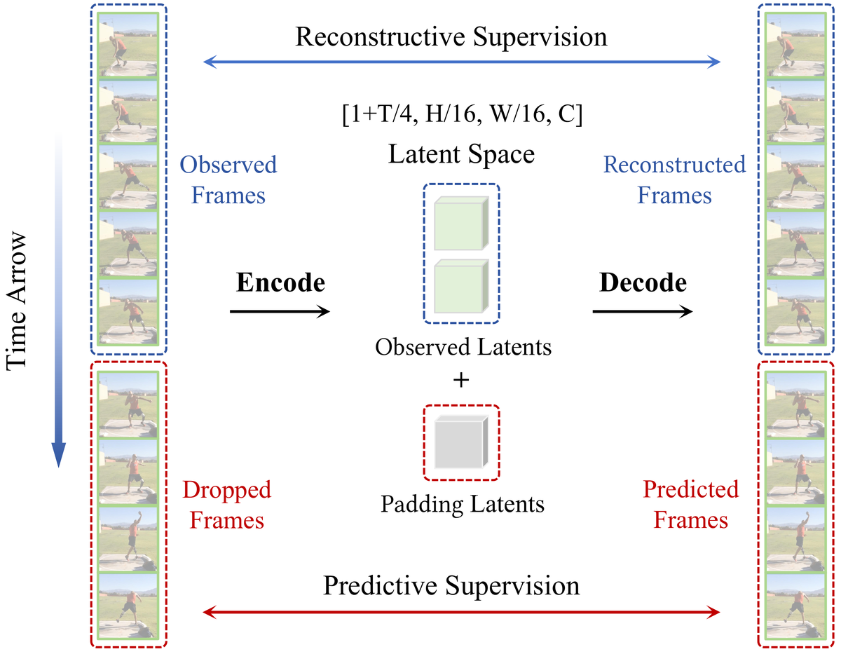
Figure 2 解读：图中上半部分是 reconstructive supervision：observed frames 被 encoder 压到 observed latents，decoder 输出 reconstructed frames；下半部分是 predictive supervision：future frames 在 encoder 输入侧被 dropped，模型只能用 observed latents 加 padding latents 组成完整 latent sequence，再预测 dropped frames。中间的 latent space 形状标为 $[1 + T /4, H /16, W /16, C]$ ，对应 PV-VAE 的 $4 \times$ temporal compression 与 $16 \times 16$ spatial compression。这个图的关键是“输入不完整、输出完整”：decoder 在训练时被迫从过去 latent 推断未来内容。

给定视频 clip $x \in R^{(1 + T) \times H \times W \times 3}$ ，采样 latent $z \in R^{(1 + t) \times h \times w \times c}$ 。空间压缩率为 $p_{s} = H / h = W / w$ ，时间压缩率为 $p_{t} = T / t$ ，额外的首帧用于统一 image/video 处理。PV-VAE 把视频沿时间切成 $G = 1 + T / p_{t}$ 个 groups，其中第一个 group 是首帧，后续每组包含 $p_{t}$ 帧。

训练时采样 dropped groups 数：

k \sim U {0, \dots, ⌊(G - 1) \cdot r ⌋},

其中 $r$ 是 maximum dropping ratio。保留前缀帧：

x_{o b s} \in R^{(1 + T - k \cdot p_{t}) \times H \times W \times 3},

encoder 得到 observed latents：

z_{o b s} \in R^{(G - k) \times h \times w \times c} .

由于 decoder 需要完整长度 latent，模型把 $z_{o b s}$ 与 $z_{p a d} \in R^{k \times h \times w \times c}$ 在时间维拼接。 $z_{p a d}$ 来自 uninformative prior，可以是 Gaussian，也可以是 learnable tokens；主实验使用 learnable padding。完整 latent 被 decoder 还原为完整视频 $\hat{x}$ 。

3.2 Key components

组件 A：Predictive Reconstruction objective。 训练目标把 reconstruction 和 prediction 合成同一个 decoder task：observed part 是标准重建，dropped part 是未来预测。直觉上，这相当于把 video VAE 从“压缩器”转成“带未来外推约束的压缩器”。如果 latent 只记住局部 texture 或静态背景，decoder 无法可靠恢复被遮掉的未来动作；因此优化会推动 encoder 把运动趋势、对象位移、动作阶段等 temporal cues 写进 latent。

组件 B：3D causal convolution VAE architecture。 PV-VAE 使用 3D causal convolutions，latent config 是 t4s16c64。Encoder 先做两阶段 spatiotemporal downsampling，把时间和空间都降 $4 \times$ ；之后保持时间长度，再做两次 spatial downsampling，最终空间总降采样 $16 \times$ 。Decoder 与 encoder 对称：先两阶段 spatial upsampling，再两阶段 spatiotemporal upsampling。

组件 C：Motion-aware objective。 论文认为预测任务容易被静态区域 copy-shortcut 稀释，因此额外要求模型重建 adjacent-frame temporal differences。这个 loss 会弱化静态背景主导的梯度，把优化压力集中到 motion boundary、relative position shift、object deformation 等真正体现 temporal evolution 的区域。

总损失为：

L_{t o t a l} = λ_{rec} (L_{MSE} + L_{D i ff}) + λ_{lp i p s} L_{L P I PS} + λ_{g an} L_{G A N} + λ_{k l} L_{K L} .

其中 $L_{D i ff}$ 是 temporal difference reconstruction，GAN loss 从 step 5,000 开启，并在 decoder fine-tuning 阶段全程开启。

组件 D：Multi-stage training。 PV-VAE 先在 256/384/512 分辨率 image data 上 pretrain 300K steps；再用 predictive reconstruction 在 256/512 video data 上 train 50K steps；最后 freeze encoder、关闭 random dropping，只 fine-tune decoder 50K steps 做标准 video reconstruction。最后一步解决训练时 decoder 常见 padding latent、推理时 latent 完整输入之间的 gap，并且不破坏已经学到的 latent diffusability。

Figure 1 解读：左侧显示 PV-VAE 在 UCF101 上相对 Wan2.2 VAE 获得 52% faster convergence 和 34.42 FVD gain；中间用 optical flow 和 point tracking probing 说明 PR 让 latent 更懂 motion；右侧 latent visualization 与 optical flow 对齐，说明 PV-VAE 的 latent 激活不只是纹理分布，而是跟视频动态结构强相关。

Figure 3 解读：上半部分比较 generation，PV-VAE 相比 Wan2.2 VAE 有更少 motion artifact、更好的 temporal coherence；下半部分比较 reconstruction，PV-VAE 保持可竞争的重建质量，但论文也指出 dense text reconstruction 仍有差距，可能来自 text-heavy samples 不足。

Figure 4 解读：该图沿 latent channel 做 PCA，并把前三个主成分可视化成 RGB。PV-VAE 的高激活区域更贴近 RAFT optical flow 中的运动区域，例如 push-up、long jump、cello hand motion、playing-card arm motion；背景区域噪声更低。这说明 PR 把 representational bandwidth 从静态背景转移到动态前景。

Figure 5 解读：Figure 5(a) 显示 frame prediction accuracy 与 generation performance 相关，支持“更会预测未来的 latent 更适合生成”；Figure 5(b) 显示 PR objective 随数据规模增大持续收益，而 pure reconstruction 没有同样趋势；Figure 5(c) 的 adjacent-frame Latent Temporal Distance 更集中、更低，表示短期更平滑；Figure 5(d) 随 frame interval 增大 LTD 单调增长，说明 latent trajectory 能表达长期 temporal dynamics。

Figure 6 解读：模型只看 observed half，却要生成完整 sequence。图中 PV-VAE 能预测被遮住未来帧的相对位置变化，红色虚线圈标出 object/background 的 relative shift。它不是简单复制最后一帧，而是在 latent 中建模动作进展。

3.3 Paper-level pseudocode

代码搜索未找到官方开源实现；以下伪代码严格按论文的 Algorithmic description、loss 与 training stages 写成，不能视为官方代码复刻。

import torch
import torch.nn.functional as F
 
 
def sample_observed_video_groups(video, pt=4, max_drop_ratio=1.0):
    # video: [B, 1 + T, C, H, W], where the first group has 1 frame
    B, total_frames, C, H, W = video.shape
    T = total_frames - 1
    G = 1 + T // pt
    max_k = int((G - 1) * max_drop_ratio)
    k = torch.randint(low=0, high=max_k + 1, size=(1,)).item()
    keep_frames = 1 + (G - k - 1) * pt
    x_obs = video[:, :keep_frames]
    x_drop = video[:, keep_frames:]
    return x_obs, x_drop, k

class PredictiveReconstructionVAE(torch.nn.Module):
    def __init__(self, encoder, decoder, latent_shape, padding="learnable"):
        super().__init__()
        self.encoder = encoder
        self.decoder = decoder
        self.padding = padding
        if padding == "learnable":
            self.pad_token = torch.nn.Parameter(torch.zeros(1, 1, *latent_shape))
 
    def pad_latents(self, z_obs, k):
        if k == 0:
            return z_obs
        B = z_obs.shape[0]
        if self.padding == "gaussian":
            z_pad = torch.randn(B, k, *z_obs.shape[2:], device=z_obs.device, dtype=z_obs.dtype)
        else:
            z_pad = self.pad_token.expand(B, k, *z_obs.shape[2:])
        return torch.cat([z_obs, z_pad], dim=1)
 
    def forward_predictive(self, video, pt=4, max_drop_ratio=1.0):
        x_obs, _, k = sample_observed_video_groups(video, pt, max_drop_ratio)
        z_obs, posterior_stats = self.encoder(x_obs)
        z_full = self.pad_latents(z_obs, k)
        recon_full = self.decoder(z_full)
        return recon_full, posterior_stats, k

def temporal_difference_loss(pred_video, target_video):
    pred_diff = pred_video[:, 1:] - pred_video[:, :-1]
    target_diff = target_video[:, 1:] - target_video[:, :-1]
    return F.mse_loss(pred_diff, target_diff)
 
 
def pv_vae_loss(pred_video, target_video, posterior_stats, perceptual_fn, discriminator=None, step=0,
                lambda_rec=1.0, lambda_lpips=1.0, lambda_gan=1.0, lambda_kl=1e-6):
    loss_mse = F.mse_loss(pred_video, target_video)
    loss_diff = temporal_difference_loss(pred_video, target_video)
    loss_lpips = perceptual_fn(pred_video, target_video).mean()
    loss_kl = posterior_stats.kl().mean()
    if discriminator is not None and step >= 5000:
        loss_gan = -discriminator(pred_video).mean()
    else:
        loss_gan = pred_video.new_tensor(0.0)
    return lambda_rec * (loss_mse + loss_diff) + lambda_lpips * loss_lpips + lambda_gan * loss_gan + lambda_kl * loss_kl

def train_pv_vae(vae, image_loader, video_loader, optimizer, perceptual_fn, discriminator):
    # Stage 1: image pretraining, 300K steps at 256/384/512 resolutions
    for step, images in enumerate(image_loader):
        pred, stats = vae.forward_standard(images)
        loss = pv_vae_loss(pred, images, stats, perceptual_fn, discriminator, step)
        loss.backward(); optimizer.step(); optimizer.zero_grad()
        if step + 1 == 300_000:
            break
 
    # Stage 2: predictive video training, 50K steps at 256/512 resolutions
    for step, videos in enumerate(video_loader):
        pred, stats, _ = vae.forward_predictive(videos, pt=4, max_drop_ratio=1.0)
        loss = pv_vae_loss(pred, videos, stats, perceptual_fn, discriminator, step)
        loss.backward(); optimizer.step(); optimizer.zero_grad()
        if step + 1 == 50_000:
            break
 
    # Stage 3: decoder fine-tuning, freeze encoder and disable dropping, 50K steps
    for p in vae.encoder.parameters():
        p.requires_grad_(False)
    for step, videos in enumerate(video_loader):
        with torch.no_grad():
            z, stats = vae.encoder(videos)
        pred = vae.decoder(z)
        loss = pv_vae_loss(pred, videos, stats, perceptual_fn, discriminator, step=5000)
        loss.backward(); optimizer.step(); optimizer.zero_grad()
        if step + 1 == 50_000:
            break

3.4 Code-to-paper mapping

Code reference: 代码搜索未找到官方开源实现；已检查论文 Project Page https://zhao-yian.github.io/PVVAE/（页面标注 Code unavailable，原因是 confidentiality constraints）、arXiv source、GitHub repository search（"Video Generation with Predictive Latents"、"PV-VAE" "Predictive Video VAE"、"PVVAE" "zhao-yian"），截至 2026-05-06 未找到可锚定的 public repo，因此不设置 github_ref。

Paper Concept	Source File	Key Class/Function
Predictive Reconstruction	未开源	论文 §3.1；上方 `sample_observed_video_groups` / `forward_predictive` 为 paper-level pseudocode
Motion-aware Objective	未开源	论文 §3.2；上方 `temporal_difference_loss` 对应 $L_{D i ff}$
Multi-stage Training	未开源	论文 §3.2；上方 `train_pv_vae` 对应 image pretrain / video PR training / decoder fine-tuning
Latte generation evaluation	未开源	论文 §4.1；仅说明移除 patchify downsampling、rectified flow 250K steps

4. Experimental Setup (实验设置)

Datasets and scale. Generation 使用 UCF101 做 class-conditional generation，RealEstate10K 做 unconditional generation；所有训练和测试视频转换为 17-frame、 $256 \times 256$ clips。Generation metrics 在 2,048 generated samples 上计算。Reconstruction 使用 Kinetics-400 validation 中随机采样的 2,048 videos，取每个视频前 17 frames，并在 $256 \times 256$ 与 $512 \times 512$ 两个分辨率评测。Latent Temporal Distance 使用 1,000 Kinetics-400 validation videos。Probing tasks 使用 Sintel（optical flow）、Kinetics-400（next-frame prediction）、TAP-Vid-DAVIS（30 videos with query points and trajectories）。

Baselines. Generation/reconstruction 主要比较 CogVideoX VAE (CogX-VAE)、IV-VAE、WF-VAE-L、HunyuanVideo VAE、Wan2.1 VAE、Wan2.2 VAE、SSVAE。Ablation 比较 Baseline、+ Predictive Reconstruction、+ Motion-aware Objective、+ Decoder Fine-tuning。Architecture discussion 中额外比较 CNN-based PV-VAE 与 Transformer-based PV-VAE♣。

Evaluation metrics. FVD / KVD 衡量 generated video distribution 与真实视频分布距离，越低越好；IS 用 C3D model 评估 UCF101 class-conditional generation 的可辨识性和多样性，越高越好；rFVD 是 reconstruction setting 下的 FVD；PSNR/SSIM 衡量像素级重建质量，越高越好；LPIPS 衡量 perceptual distance，越低越好；EPE 是 optical flow endpoint error，越低越好；MSE 是 next-frame prediction error，越低越好；AUC 是 point tracking 在 0–10 pixels threshold 下的 tracking accuracy area，越高越好；LTD 是 latent temporal distance，用 latent 的平均 L2 distance 衡量时间连续性。

Training config. PV-VAE 使用 AdamW，base learning rate $5 \times 1 0^{- 5}$ ，linear warmup，cosine schedule 中学习率衰减 10 倍；random dropping 固定保留首帧，maximum dropping ratio $r = 1.0$ 。VAE image pretraining 300K steps，video predictive training 50K steps，decoder fine-tuning 50K steps。Generation model 使用 Latte architecture，移除 patchify downsampling，rectified flow 训练 250K steps，learning rate $1 \times 1 0^{- 4}$ ，global batch size 64，Euler sampler 100 steps。速度/显存指标在 17-frame $256 \times 256$ clips、batch size 4 下测量，100 steps 平均，前 50 warm-up steps。论文正文未详细说明 GPU 型号/数量；项目页版本的 snippet 提到实验使用 16 NVIDIA H800 GPUs，速度显存用 single NVIDIA H20 GPU 测量，但 arXiv PDF 正文未保留该句，因此这里以 PDF 为准标记为“论文未详细说明”。

5. Experimental Results (实验结果)

Main generation results (Table 1, 17-frame $256 \times 256$ ).

Method	Latent config	UCF101 FVD↓	UCF101 KVD↓	UCF101 IS↑	RealEstate10K FVD↓	RealEstate10K KVD↓	TSpeed it/s	TMem GiB	Param M
CogX-VAE	t4s8c16	176.90	16.47	64.19	94.12	10.41	0.76	85.93	216
IV-VAE	t4s8c16	175.74	22.32	64.51	92.37	8.35	1.28	88.34	242
WF-VAE-L	t4s8c16	188.19	33.01	67.49	107.26	12.56	2.52	87.36	317
Hunyuan-VAE	t4s8c16	210.30	52.81	66.40	83.45	13.23	1.64	87.36	246
Wan2.1 VAE	t4s8c16	167.10	11.54	66.04	83.84	10.64	1.88	86.44	127
Wan2.2 VAE	t4s16c48	180.79	17.80	67.32	87.15	10.11	4.96	30.90	705
SSVAE	t4s16c48	168.68	19.71	66.39	79.08	8.79	3.92	34.00	315
PV-VAE	t4s16c64	146.37	14.52	69.72	72.50	4.06	4.40	33.34	661

PV-VAE 在 UCF101 FVD 上比 Wan2.2 VAE 低 34.42，比 SSVAE 低 22.31；比 Hunyuan-VAE 低 63.93，同时 training speed 提升到 4.40 it/s（相对 Hunyuan-VAE 2.68×），TMem 从 87.36 GiB 降到 33.34 GiB。RealEstate10K 上 PV-VAE 也取得最低 FVD 72.50 和最低 KVD 4.06。

Reconstruction results (Table 2, Kinetics-400 validation).

Method	17×256 rFVD↓	PSNR↑	SSIM↑	LPIPS↓	17×512 rFVD↓	PSNR↑	SSIM↑	LPIPS↓	ISpeed it/s	IMem GiB
CogX-VAE	4.90	33.78	0.97	0.027	1.79	36.00	0.99	0.024	0.46	13.64
IV-VAE	2.78	34.08	0.96	0.019	0.97	37.24	0.96	0.016	0.32	5.39
WF-VAE-L	3.06	33.48	0.96	0.023	1.08	35.93	0.96	0.023	0.87	5.00
Hunyuan-VAE	2.96	34.30	0.97	0.016	0.90	37.13	0.97	0.015	0.50	22.00
Wan2.1 VAE	2.92	33.21	0.95	0.018	1.02	36.15	0.97	0.017	0.60	6.77
Wan2.2 VAE	3.42	33.78	0.96	0.015	1.22	36.75	0.97	0.015	0.58	9.36
SSVAE	7.50	31.18	0.96	0.036	2.16	34.45	0.97	0.028	0.64	7.63
PV-VAE	3.45	32.26	0.95	0.020	1.88	35.03	0.97	0.020	0.69	7.97

Reconstruction 不是 PV-VAE 的单点最优：它在 256 rFVD 上接近 Wan2.2 VAE（3.45 vs. 3.42），但 PSNR/LPIPS 略低；相比 SSVAE 则稳定更好。论文强调这正说明 generation-ready latent 不等于 reconstruction-optimal latent。

Latent/video understanding probing (Table 3).

Method	EPE↓	MSE↓	AUC(%)↑
w/o PR	5.9223	0.0314	70.95
w/ PR	5.1805 (+12.5%)	0.0289 (+8.0%)	76.99 (+8.5%)

第 14 层（共 28 层）LVDM diffusion features 用于 optical flow、next-frame prediction、point tracking 三个 probe。PV-VAE 在三项任务均提升，说明 PR 改善的不是单纯的 FVD trick，而是 latent 中的 video dynamics representation。

Ablation results (Tables 4–6).

Configuration	gFVD↓	rFVD↓	PSNR↑	SSIM↑	LPIPS↓
Baseline	174.81	3.03	33.44	0.96	0.017
+ Predictive Reconstruction	156.33	5.66	31.47	0.94	0.026
+ Motion-aware Objective	150.10	5.79	31.38	0.94	0.026
+ Decoder Fine-tuning	146.37	3.45	32.26	0.95	0.020

PR 直接把 gFVD 从 174.81 降到 156.33，但牺牲 reconstruction；motion-aware objective 继续把 gFVD 降到 150.10；decoder fine-tuning 把 rFVD 从 5.79 拉回 3.45，并进一步把 gFVD 降到 146.37。

MDR	gFVD↓	KVD↓	IS↑
50%	159.82	14.67	69.35
75%	154.06	16.93	70.27
100%	146.37	14.52	69.72

更大的 maximum dropping ratio 带来更强 predictive regularization，UCF101 gFVD 最优出现在 100%。

Padding	gFVD↓	KVD↓	IS↑
Gaussian	150.68	11.87	68.01
Learnable	146.37	14.52	69.72

Learnable padding 在 gFVD/IS 上更好，但 Gaussian padding 的 KVD 更低；主结果选择 learnable padding。

Transformer VAE discussion (Table 7).

Model	UCF101 gFVD↓	KVD↓	IS↑	Kinetics rFVD↓	PSNR↑	SSIM↑	LPIPS↓	ISpeed it/s
PV-VAE	146.37	14.52	69.72	3.45	32.26	0.95	0.020	0.69
PV-VAE♣	178.86	20.66	69.80	4.03	33.02	0.95	0.022	1.29

Transformer-based variant 有 12-layer encoder、12-layer decoder、16 heads、128 head_dim、约 1.2B parameters，推理速度 1.29 it/s，比 CNN PV-VAE 快 87%，但 generative capability 仍明显弱于 CNN 版本（gFVD 178.86 vs. 146.37）。作者把它作为未来方向，而非当前最佳设计。

Limitations. 作者明确提到 PV-VAE 在 dense text reconstruction 上有 subtle limitations，可能因为当前数据分布中 text-heavy samples 较少；另外 Transformer-based video VAE 虽然更快，但 generation gap 仍大。论文也暗示 reconstruction/generation trade-off 仍是 tokenizer 设计核心矛盾：高维丰富 latent 有利于细节，但如果没有结构化先验，会使生成更困难。

Overall conclusion. PV-VAE 证明 video VAE 的目标不应只追求 reconstruction fidelity，而应让 latent 学到 temporal predictive structure。Predictive Reconstruction、motion-aware objective 和 decoder fine-tuning 组合后，模型在 UCF101 / RealEstate10K generation 上显著优于现有 Video VAEs，并在多项 video understanding probes 中展现更强 motion-aware representation。

Paper Notes

探索

Video Generation with Predictive Latents

Video Generation with Predictive Latents

1. Motivation (研究动机)

2. Idea (核心思想)

3. Method (方法)

3.1 Overall framework

3.2 Key components

3.3 Paper-level pseudocode

3.4 Code-to-paper mapping

4. Experimental Setup (实验设置)

5. Experimental Results (实验结果)

目录