Resampling Forcing: End-to-End Training for Autoregressive Video Diffusion via Self-Resampling

1. Motivation (研究动机)

核心问题: Autoregressive 视频扩散模型的 Exposure Bias

自回归(AR)视频扩散模型通过逐帧生成来模拟视频的因果结构，具有天然的世界模型潜力。但其训练和推理存在严重的 train-test mismatch:

• 训练时 (Teacher Forcing): 模型以 ground truth 历史帧为条件预测当前帧
• 推理时: 模型以自己生成的(不完美的)历史帧为条件

这导致 error accumulation — 模型误差在自回归 rollout 中逐帧累积放大，最终造成视频质量崩溃(颜色失真、纹理退化、内容漂移)。

现有方案的局限

方案	代表工作	局限性
后训练蒸馏	Self Forcing, CausVid, LongLive	依赖 14B 双向 teacher 模型，无法从头训练；teacher 泄露未来信息，破坏因果性
在线判别器	对抗训练方法	训练不稳定，扩展性差
噪声注入	noise augmentation	噪声分布与真实模型误差不匹配
滑窗注意力	sliding window	丢失长程依赖，加剧 drift

核心 Motivation: 能否设计一种 无需 teacher、无需判别器 的端到端训练方法，从头训练出鲁棒的 AR 视频扩散模型？

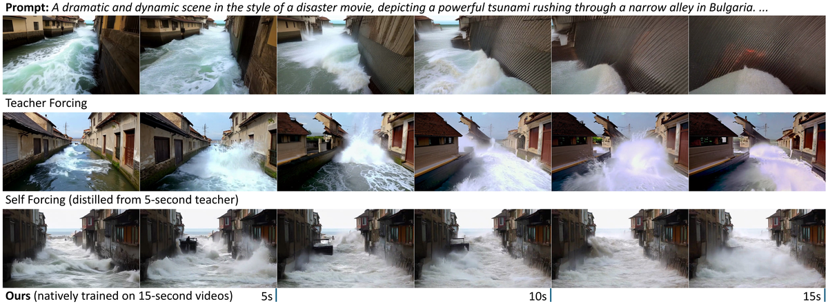
Figure 1 解读: 对比三种训练策略在生成 15 秒长视频时的效果。Top: Teacher Forcing 训练的模型随时间积累误差，最终视频崩溃。Middle: Self Forcing 从 5 秒 bidirectional teacher 蒸馏，在长视频上质量退化。Bottom: Resampling Forcing 原生在 15 秒视频上训练，全程保持稳定的视觉质量和时间一致性。

---

2. Idea (核心思想)

核心思想: Self-Resampling 模拟推理误差

Resampling Forcing 的核心洞察非常简洁:

训练时主动在历史帧上引入模型自身的误差，然后让模型学会在这些”退化”历史帧条件下仍能正确预测干净目标。

具体而言:

1. Self-Resampling: 用在线模型对 ground truth 历史帧进行部分去噪重采样，模拟推理时的模型误差
2. Autoregressive Error Propagation: 重采样过程是自回归的 — 每一帧的退化依赖于前面已退化帧的条件，准确模拟推理时的误差累积模式
3. Clean Target, Degraded Condition: 条件(历史)是退化的，但预测目标始终是干净的 ground truth

这使得模型学会了 error correction 而非 error amplification，从而在推理时将误差控制在近似恒定水平。

Figure 2 解读: 误差累积机制对比。Top (Teacher Forcing): 训练时用完美输入，推理时模型误差逐帧累积放大，分布偏移越来越严重。Bottom (Ours): 训练时用含模拟误差的历史帧，模型学会修正输入误差，推理时误差被限制在近似恒定范围内，不再累积。灰色圆圈代表 ground truth 分布中的最近匹配点。

---

3. Method (方法)

3.1 背景: AR 视频扩散模型

给定条件 $c$，$N$ 帧视频 ${\mathbf{x}}^{1:N}$ 的联合分布分解为自回归形式:

$$p({\mathbf{x}}^{1:N}|c)=\prod _{i=1}^{N}p({\mathbf{x}}^i|{\mathbf{x}}^{<i},c)$$

每帧通过求解反向 ODE 从噪声 ${\mathbf{x}}_1^i\sim \mathcal{N}(0,\mathbf{I})$ 生成:

$${\mathbf{x}}^i={\mathbf{x}}_1^i+{\int }_1^0{\mathbf{v}}_{\theta }({\mathbf{x}}_t^i,{\mathbf{x}}^{<i},t,c)\mathrm{d}t$$

其中 ${\mathbf{v}}_{\theta }$ 是 velocity field 网络 (DiT 架构)，使用 Flow Matching 训练。

3.2 Teacher Forcing 训练

在 Flow Matching 框架下，时刻 $t$ 的样本为:

$${\mathbf{x}}_t^i=(1-t)\cdot {\mathbf{x}}^i+t\cdot {\mathbf{ϵ}}^i$$

训练目标为回归 velocity $\mathrm{d}{\mathbf{x}}_t^i/\mathrm{d}t={\mathbf{ϵ}}^i-{\mathbf{x}}^i$:

$$\mathcal{L}={\mathbb{E}}_{i,t,\mathbf{x},\mathbf{ϵ}}\left[\Vert ({\mathbf{ϵ}}^i-{\mathbf{x}}^i)-{\mathbf{v}}_{\theta }({\mathbf{x}}_t^i,{\mathbf{x}}^{<i},t,c){\Vert }_2^2\right]$$

通过 causal mask 实现所有帧的并行训练。

3.3 Resampling Forcing 核心方法

3.3.1 Autoregressive Self-Resampling

为模拟推理时的两类误差 — (1) 帧内去噪不完美导致的高频细节误差，(2) 帧间自回归累积误差 — 提出 autoregressive self-resampling:

对每帧 ground truth ${\mathbf{x}}^i$:

1. 采样 simulation timestep $t_s\in (0,1)$，将其加噪到 ${\mathbf{x}}_{t_s}^i$
2. 用在线模型 ${\mathbf{v}}_{\theta }$ 从 $t_s$ 完成剩余去噪，得到退化帧 ${\tilde{\mathbf{x}}}^i$

$${\tilde{\mathbf{x}}}^i={\mathbf{x}}_{t_s}^i+{\int }_{t_s}^0{\mathbf{v}}_{\theta }({\mathbf{x}}_t^i,{\tilde{\mathbf{x}}}^{<i},t,c)\mathrm{d}t$$

关键设计:

• 自回归条件: 重采样时以已退化的 ${\tilde{\mathbf{x}}}^{<i}$ 为条件，精确模拟推理时误差累积
• 在线权重: 使用当前训练中的模型权重，使误差分布随训练动态演化
• 梯度截断: 重采样过程 stop gradient，防止模型学会捷径(shortcut learning)

3.3.2 Simulation Timestep 采样策略

$t_s$ 控制重采样强度的 trade-off:

• $t_s\to 0$: 退化帧接近 ground truth (退化为 teacher forcing)
• $t_s\to 1$: 退化强但可能导致内容漂移

采样分布选择 Logit-Normal:

$$\text{logit}(t_s)\sim \mathcal{N}(0,1)$$

并应用 timestep shifting (参数 $s$) 偏向低噪声区:

$$t_s\leftarrow s\cdot t_s/(1+(s-1)\cdot t_s)$$

实验中 $s=0.6$，即适度偏向低噪声(弱退化)。

3.3.3 Sparse Causal Mask 并行训练

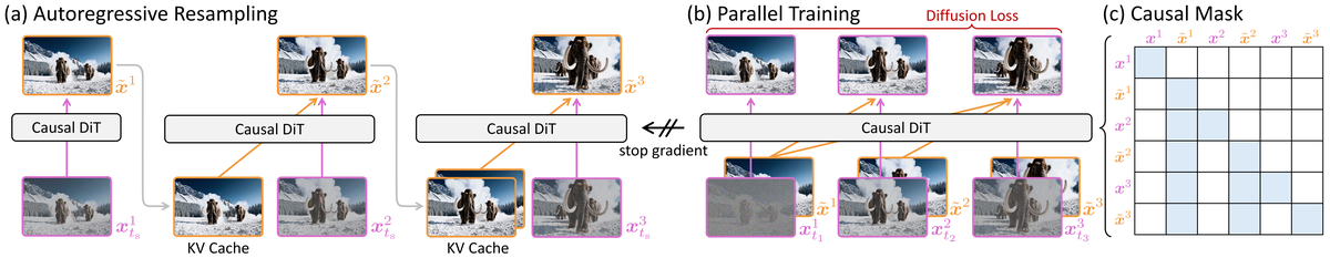
Figure 3 解读: Resampling Forcing 方法全览。(a) Autoregressive Resampling: 对 ground truth 帧加噪到 $t_s$，然后用在线模型自回归地完成去噪，生成含模型误差的退化帧，通过 KV Cache 实现高效推理。(b) Parallel Training: 退化帧作为历史条件 (stop gradient)，所有帧在一次前向传播中并行计算 frame-level diffusion loss。(c) Causal Mask: 稀疏因果掩码确保每帧只能 attend 到自身的噪声版本和前面帧的干净版本，维持因果性。

训练流程分两步:

1. 重采样阶段 (no gradient): 自回归生成退化历史 ${\tilde{\mathbf{x}}}^{1:N}$
2. 训练阶段 (with gradient): 以 ${\tilde{\mathbf{x}}}^{<i}$ 为条件，并行计算所有帧的 diffusion loss

$$\mathcal{L}=\frac{1}{N}\sum _{i=1}^N\Vert ({\mathbf{ϵ}}^i-{\mathbf{x}}^i)-{\mathbf{v}}_{\theta }({\mathbf{x}}_{t_i}^i,{\tilde{\mathbf{x}}}^{<i},t_i,c){\Vert }_2^2$$

3.3.4 Teacher Forcing Warmup

训练初期模型尚未收敛，self-resampling 产生的误差无意义。因此先用 Teacher Forcing 预热 10K steps，再切换到 Resampling Forcing。

3.4 History Routing: 动态稀疏注意力

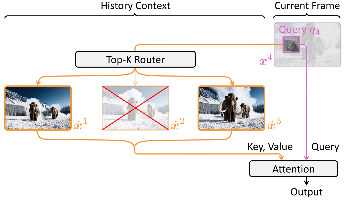
Figure 4 解读: History Routing 机制。当生成第 4 帧时，不是 attend 到所有历史帧 (dense causal attention)，而是通过 Top-K Router 动态选择最相关的 $k$ 帧 (图中 $k=2$，选择了第 1、3 帧)。每个 query token 独立路由，不同 head 和位置可选择不同的历史帧，实际有效感受野远大于 $k$。

随着生成帧数增长，dense causal attention 的 KV 数量线性增长，计算量暴增。提出 History Routing 替代:

对 query token ${\mathbf{q}}_i$，动态选择 top-$k$ 最相关历史帧:

$$\text{Attention}({\mathbf{q}}_i,{\mathbf{K}}_{<i},{\mathbf{V}}_{<i})=\text{Softmax}\left(\frac{{\mathbf{q}}_i{\mathbf{K}}_{\Omega ({\mathbf{q}}_i)}^{\top }}{\sqrt{d}}\right)\cdot {\mathbf{V}}_{\Omega ({\mathbf{q}}_i)}$$

其中 $\Omega ({\mathbf{q}}_i)$ 是为 query ${\mathbf{q}}_i$ 选择的 $k$ 个历史帧索引集合:

$$\Omega ({\mathbf{q}}_i)=\arg \underset{{\Omega }^{\ast }}{\max }\sum _{j\in {\Omega }^{\ast }}({\mathbf{q}}_i^{\top }\varphi ({\mathbf{K}}_j))$$

$\varphi (\cdot )$ 为 mean pooling (无参数)，将每帧的 KV 池化为 frame descriptor。

实现细节:

• 采用 MoBA 风格的双分支注意力: intra-frame branch + history branch
• 通过 global log-sum-exp 融合两个分支输出
• 使用 flash_attn_varlen_func() 高效实现
• 注意力稀疏度 $1-k/L$，$k=5$ 时对 20 帧历史实现 75% 稀疏度
• 路由是 head-wise 和 token-wise 的，不同 head/position 可选不同帧

3.5 完整算法伪码

# Resampling Forcing
 
> **Authors**: Yuwei Guo, Ceyuan Yang, Hao He, Yang Zhao, Meng Wei, Zhenheng Yang, Weilin Huang, Dahua Lin
> **Affiliations**: The Chinese University of Hong Kong, ByteDance Seed, ByteDance
> **GitHub**: [guandeh17/Self-Forcing](https://github.com/guandeh17/Self-Forcing)
> **Venue**: ICCV 2025
 
while not converged:
    t_s = sample_logit_normal()
    t_s = shift_timestep(t_s, s)
    clean_video, condition = sample_batch(dataset)
    noisy_video = add_noise(clean_video, t_s)
 
    with no_grad():
        degraded_history = autoregressive_self_resampling(
            model=v_theta,
            clean_video=clean_video,
            t_s=t_s,
            condition=condition,
        )
 
    sampled_steps = sample_training_steps(num_frames=len(clean_video))
    loss = 0.0
    for frame_idx, t_i in enumerate(sampled_steps):
        eps_i = torch.randn_like(clean_video[frame_idx])
        x_t_i = add_noise(clean_video[frame_idx], t_i, noise=eps_i)
        target = eps_i - clean_video[frame_idx]
        pred = v_theta(x_t_i, degraded_history[:frame_idx], t_i, condition)
        loss += mse(pred, target)
 
    loss /= len(clean_video)
    optimize(loss, params=theta)
 
return theta

3.6 Resampling 过程伪码

def autoregressive_self_resampling(model, clean_video, t_s, condition):
    """
    模拟推理时的模型误差
    Args:
        model: 在线 v_θ 模型
        clean_video: ground truth x^{1:N}, shape [N, C, H, W]
        t_s: simulation timestep (scalar)
        condition: text condition c
    Returns:
        degraded_video: 退化视频 x̃^{1:N}
    """
    N = clean_video.shape[0]
    noise = torch.randn_like(clean_video)
 
    # 加噪到 t_s
    noisy_video = (1 - t_s) * clean_video + t_s * noise  # [N, C, H, W]
 
    degraded_video = []
    kv_cache = None
 
    with torch.no_grad():  # 关键: stop gradient
        for i in range(N):
            # 1-step Euler 近似从 t_s 到 0
            x_t = noisy_video[i]
            history = degraded_video  # 已退化的前置帧
 
            velocity = model(x_t, history, t_s, condition)
            x_clean = x_t + (0 - t_s) * velocity  # Euler step
 
            degraded_video.append(x_clean)
            # 更新 KV cache
 
    return torch.stack(degraded_video)

3.7 History Routing 伪码

def history_routing_attention(query, kv_cache, k=5):
    """
    动态 Top-K History Routing
    Args:
        query: 当前帧的 query tokens, shape [num_tokens, d]
        kv_cache: 历史帧 KV, list of (K_j, V_j) each [tokens_per_frame, d]
        k: 选择的历史帧数
    Returns:
        attention output
    """
    num_history = len(kv_cache)
    if num_history <= k:
        # 历史帧不够 k 个，使用全部
        return dense_attention(query, kv_cache)
 
    # Step 1: 计算 frame descriptors (mean pool, 无参数)
    frame_descriptors = []
    for K_j, V_j in kv_cache:
        phi_j = K_j.mean(dim=0)  # [d], mean pooling
        frame_descriptors.append(phi_j)
    frame_descriptors = torch.stack(frame_descriptors)  # [L, d]
 
    # Step 2: Per-token routing score
    scores = query @ frame_descriptors.T  # [num_tokens, L]
 
    # Step 3: Top-K selection (per token)
    _, topk_indices = scores.topk(k, dim=-1)  # [num_tokens, k]
 
    # Step 4: Gather selected KVs and compute attention
    # 实际使用 flash_attn_varlen_func 高效实现
    output = sparse_attention(query, kv_cache, topk_indices)
 
    # Step 5: 融合 intra-frame 和 history 分支 (log-sum-exp)
    intra_output = intra_frame_attention(query)
    final_output = logsumexp_fusion(intra_output, output)
 
    return final_output

---

4. Experimental Setup (实验设置)

4.1 模型配置

配置项	详情
基础模型	WAN2.1-1.3B (DiT 架构)
分辨率	480 x 832
原始能力	5 秒 (81 帧) 双向注意力
Chunk size	3 latent frames (自回归单元)
Causal mask	torch.flex_attention() 实现，无额外参数
Timestep conditioning	修改为支持 per-frame noise level

4.2 训练配置

阶段	视频长度	Steps	说明
Stage 1: Teacher Forcing warmup	5s	10K	切换为 causal attention 后预热
Stage 2: Resampling Forcing	5s	15K	开始 self-resampling
Stage 3: Resampling Forcing	15s (249 帧)	5K	原生长视频训练
Stage 4: Fine-tune w/ History Routing	15s	1.5K	启用 sparse attention

超参数	值
Batch size	64
Optimizer	AdamW
Learning rate	5e-5
Timestep shift $s$	0.6
History routing $k$	5
Resampling solver	1-step Euler

4.3 推理配置

配置项	值
Sampler	Euler, 32 steps
Timestep shifting factor	5.0
CFG scale	5.0

4.4 评测

• Benchmark: VBench
• 视频长度: 15 秒，分三段 (0-5s, 5-10s, 10-15s) 分别评测
• 指标: Temporal Quality, Visual Quality, Text Alignment
• Baselines: SkyReels-V2 (1.3B), MAGI-1 (4.5B), NOVA (0.6B), Pyramid Flow (2.0B), CausVid (1.3B), Self Forcing (1.3B), LongLive (1.3B)

---

5. Experimental Results (实验结果)

5.1 定量结果 (VBench, 15s 视频)

Table 1: 主要对比结果

Method	Param	Teacher Model	0-15s Temp	0-15s Vis	0-15s Text	5-10s Temp	10-15s Temp
SkyReels-V2	1.3B	-	81.93	60.25	21.92	84.63	87.50
MAGI-1	4.5B	-	87.09	59.79	26.18	89.10	86.66
NOVA	0.6B	-	87.58	44.42	25.47	88.40	84.94
Pyramid Flow	2.0B	-	81.90	62.99	27.16	84.45	84.27
CausVid	1.3B	WAN2.1-14B(5s)	89.35	65.80	23.95	89.59	87.14
Self Forcing	1.3B	WAN2.1-14B(5s)	90.03	67.12	25.02	84.27	84.26
LongLive	1.3B	WAN2.1-14B(5s)	81.84	66.56	24.41	81.72	84.57
Ours (75% sparsity)	1.3B	-	90.18	63.95	24.12	89.80	87.03
Ours	1.3B	-	91.20	64.72	25.79	90.44	89.74

关键发现:

• 无需 teacher 模型即达到与蒸馏方法 (CausVid, Self Forcing) 可比的质量
• Temporal Quality 全面领先 (91.20 vs Self Forcing 90.03)，尤其在长视频段 (10-15s) 优势显著 (89.74 vs 84.26)
• 75% 稀疏度下质量几乎无损 (90.18 vs 91.20 Temporal)
• 蒸馏方法在长视频段 temporal 指标显著下降 (Self Forcing: 90.03→84.26)，说明短 teacher 泄露的未来信息导致因果性问题

5.2 定性对比

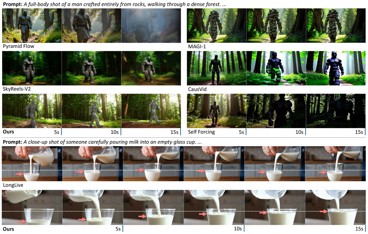
Figure 5 解读: 定性比较。Top panel: 在 “岩石人行走” prompt 上，Pyramid Flow/CausVid/Self Forcing 均出现颜色/纹理退化，而本方法 15 秒全程质量稳定。MAGI-1 和 SkyReels-V2 虽然长视频退化较轻，但牺牲了严格因果性。Bottom panel: 在 “倒牛奶” prompt 上，从 5 秒 bidirectional teacher 蒸馏的 LongLive 出现液位先升后降的非因果现象 (红色箭头)，违反物理规律。本方法严格因果训练，液位单调上升，符合物理一致性。

5.3 消融实验

误差模拟策略 (Table 2)

Strategy	Temporal	Visual	Text
Noise augmentation	87.15	61.90	21.44
Resampling - parallel	88.01	62.51	24.51
Resampling - autoregressive	90.46	64.25	25.26

结论: 自回归重采样显著优于并行重采样和噪声增强，因为它准确模拟了推理时误差的 累积模式。

Timestep Shifting 因子 $s$

Figure 6 解读: 不同 shift 因子 $s$ 对生成质量的影响。$s=0.1$ (轻微退化): 模型仍然积累误差，质量退化。$s=0.6$ (适中): 平衡误差鲁棒性和内容保真度。$s=3.0$ (强退化): 模型过度偏离历史内容，出现内容漂移 (如气球形态变化)。因此需要适中的 $s$ 值。

稀疏历史策略

Figure 7 解读: 四种历史注意力策略对比。Dense Causal Attention 效果最好但计算量线性增长。History Routing top-5 (75% 稀疏) 质量接近 dense，显著优于 Sliding Window (size=1) 和 top-1 routing。即使 top-1 (95% 稀疏) 也优于等价稀疏度的 sliding window，说明动态路由比固定窗口能选择更有信息量的上下文。

History Routing 频率分析

Figure 8 解读: 生成第 21 帧时，前 20 帧被路由选中的频率分布。呈现 “sliding window + attention sink” 的混合模式 — 模型优先关注最近的帧和初始帧 (anchor frames)。$k=1$ 时这种模式最极端，$k$ 增大后选择更均匀，覆盖中间帧。这验证了近期 “frame sinks + sliding window” 注意力设计是 dynamic routing 的一个特例。

5.4 代码-论文对应关系

由于 Resampling Forcing 尚未开源，以下基于相关工作 Self Forcing (github.com/guandeh17/Self-Forcing) 的代码结构进行推测性映射:

论文组件	推测代码位置	说明
AR Video Diffusion Model	model/	基于 WAN2.1 的 DiT 架构，需添加 per-frame timestep conditioning
Causal Mask	model/ 或 wan/	论文使用 torch.flex_attention() 实现 sparse causal mask
Self-Resampling	trainer/	训练循环中 no-grad 阶段，自回归调用模型生成退化帧
KV Cache	model/ + pipeline/	重采样和推理共用的 KV cache 机制
History Routing	model/ attention layers	Top-K 路由 + flash_attn_varlen_func() 双分支注意力
Training Loop	trainer/ + train.py	两阶段: resampling (no grad) → parallel training (grad)
Euler Solver	pipeline/	推理 32 steps Euler；重采样 1-step Euler
Timestep Shifting	trainer/ 或 utils/	LogitNormal 采样 + shift 公式

---

总结

Resampling Forcing 提出了一种优雅的 teacher-free 端到端训练框架:

1. Self-Resampling 用在线模型自身的误差替代外部 teacher 信号，是对 Scheduled Sampling (NLP) 思想在 diffusion 领域的精妙适配
2. Autoregressive Error Simulation 准确模拟推理时的误差累积模式，优于简单噪声增强或并行重采样
3. History Routing 以无参数 top-K 路由实现近恒定注意力复杂度，且路由自动学到了 “attention sink + sliding window” 模式
4. 整体方法简洁、不引入额外参数或模型，在 1.3B 模型上即达到需要 14B teacher 的蒸馏方法的可比质量，且在长视频因果一致性上更优