When Does LeJEPA Learn a World Model?

Paper: arXiv:2605.26379 Code: klindtlab/lejepa-identifiability Code reference: main @ de7503f1 (2026-05-27)

1. Motivation (研究动机)

这篇论文要回答一个非常尖锐的问题：JEPA / LeJEPA 学到的 latent representation 什么时候真的可以叫 World Model，而不只是一个对下游任务有用的 embedding？作者把“真的学到世界”定义成 linear identifiability：学到的表示 $h(z)$ 必须能通过一个线性正交变换恢复真实 latent variables $z$，而不是把位置、颜色、速度、纹理等自由度非线性地缠在一起。

现有 JEPA 系列方法的主要问题不是“能否避免 collapse”这么简单。I-JEPA、V-JEPA、LeJEPA、LeWorldModel 等方法已经能通过 alignment loss、variance/covariance regularization 或 Gaussian regularization 训练出稳定表示；但这些经验 recipe 只能说明 embedding 不坍缩、预测损失小，并不能证明表示保留了世界的真实自由度。如果一个 representation 把两个独立 latent 以非线性方式混合，它依然可能在局部预测或 probe 上表现不错，却会在 planning、compositional generalization 或 out-of-distribution 组合时失败。

论文特别关心 LeJEPA，因为 LeJEPA 把 collapse prevention 明确写成“embedding distribution 接近 isotropic Gaussian”的 SIGReg 约束。这个显式 distributional constraint 让理论分析成为可能：如果正样本来自一个 stationary additive-noise world，且真实 latent 是 Gaussian，那么 alignment + Gaussianity 是否足够把未知非线性观测 $x=g(z)$ 逆回来？反过来，如果真实 latent 不是 Gaussian，同样的 recipe 是否还保证 linear recovery？

研究这个问题的价值在于：World Model 的核心用途是 planning，而 planning 不只需要“相似状态靠近”，还需要 latent 坐标几何和真实状态空间几何一致。若 $h(z)=Qz$ 且 $Q$ 是 orthogonal transformation，那么在 learned latent space 里做最短路、控制代价、value function 等操作不会被 representation distortion 破坏；若 $h$ 是任意非线性 map，latent-space straight line 可能对应真实空间里的弯曲甚至无效轨迹。

2. Idea (核心思想)

核心洞察是：在 Gaussian OU world 中，positive-pair alignment 实际上是在最大化跨时间相关性，而 Gaussian 下的 transition operator 的 eigenfunctions 正是 Hermite polynomials；线性 Hermite 分量的相关性衰减是 $\rho$，任何二阶及以上非线性分量只能得到 ${\rho }^2,{\rho }^3,\dots$，因此只要 embedding 被约束成 isotropic Gaussian，最优解就必须把所有方差放在线性分量上。

换句话说，LeJEPA 的 Gaussian regularization 不是普通的 anti-collapse trick，而是把可行解限制到“分布正确”的表示族；alignment loss 则在这个族里惩罚所有非线性扭曲。两者合起来迫使 $h=f\circ g$ 成为真实 latent 的 rotation/reflection：$h(z)=Qz$。

与传统 ICA / nonlinear ICA 的差异在于，ICA 通常依赖非高斯性来识别 independent components；这篇论文反过来证明，在 stationary additive-noise world + LeJEPA objective 下，Gaussian 是唯一能保证 linear identifiability 的 latent distribution。与 LeJEPA: Provable and Scalable Self-Supervised Learning Without the Heuristics 或 LeWorldModel: Stable End-to-End Joint-Embedding Predictive Architecture from Pixels 相比，本文不是再提出一个训练 recipe，而是给出该 recipe 何时真正学到 World Model 的充分且近似必要条件。

3. Method (方法)

3.1 Overall framework：world、nonlinear observation、LeJEPA representation

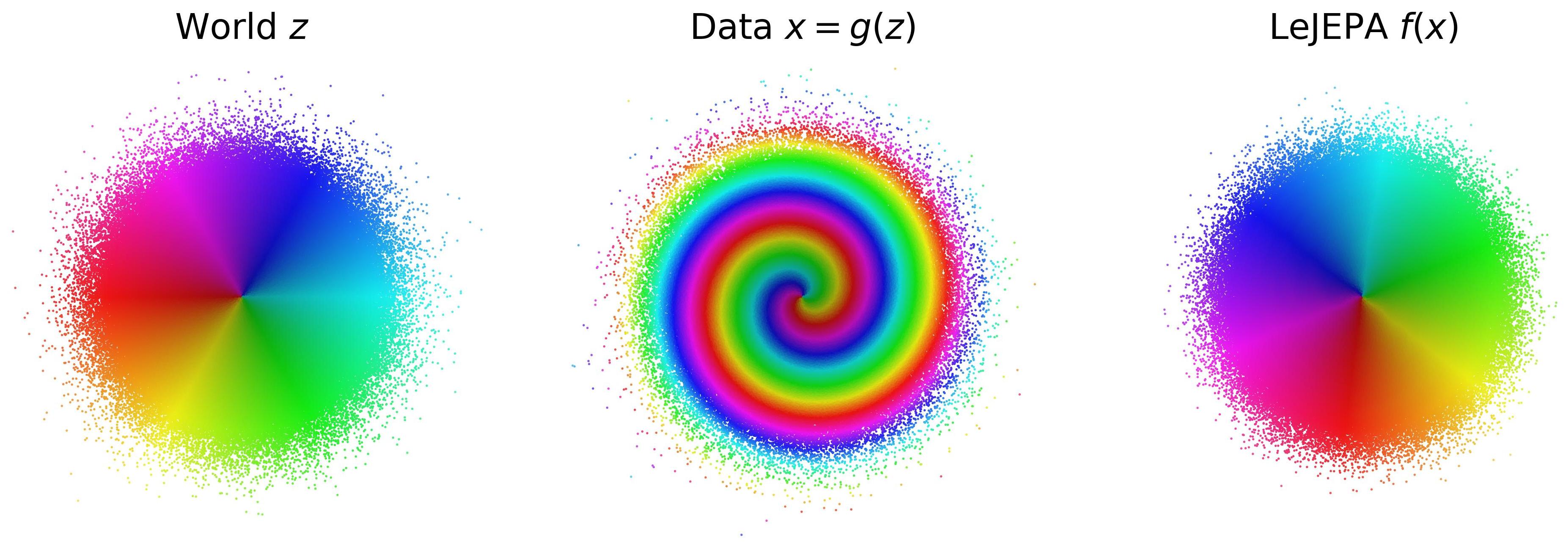
Figure 1 解读：左侧是真实世界的 latent variables $z$，组件独立且服从 Gaussian；中间是未知非线性观测过程 $x=g(z)$，它把原本干净的自由度扭曲成复杂观测；右侧是 LeJEPA 通过 encoder $f$ 学到的表示 $h=f\circ g$。论文要证明的是，在合适条件下右侧不是任意好看的 embedding，而是左侧 latent 的 rotation/reflection，因此仍然保留世界的线性结构。

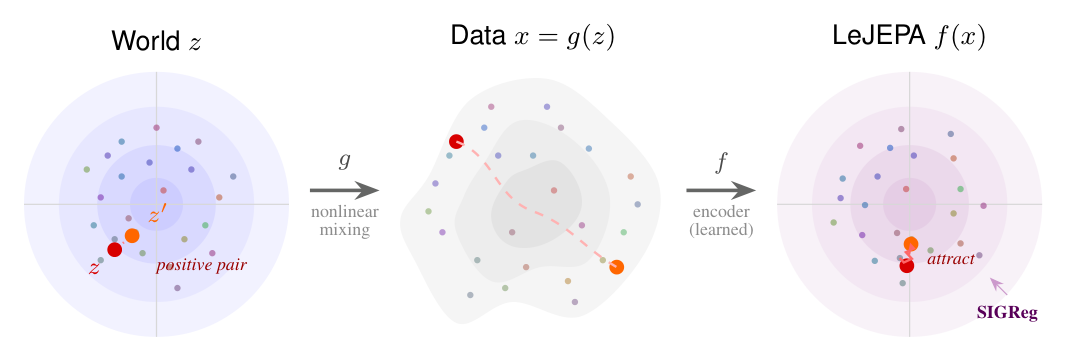
Figure 2 解读：这张图把理论对象和训练目标对齐起来：world 产生 correlated positive pair $(z,z^{\prime })$，未知 $g$ 把它们变成 observation pair $(x,x^{\prime })$，LeJEPA 用 alignment 把 positive pair 拉近，同时用 SIGReg 让 embedding distribution 保持 Gaussian。PDF 中该图由 LaTeX/TikZ 绘制，arXiv source 没有独立图片文件；笔记中使用 page-level diagram crop 作为 source-first extraction 的唯一记录型 fallback。

方法可以写成一个三层组合：

• World：真实 latent $z\in {\mathbb{R}}^n$ 生成正样本对 $(z,z^{\prime })$，并满足 independence、stationarity、additive noise。
• Observation：观测是未知非线性混合 $x=g(z)$，训练者只看到 $(x,x^{\prime })=(g(z),g(z^{\prime }))$。
• Learner：encoder $f$ 产生 $h=f\circ g$，目标是让 $h(z)$ 在分布上接近 $\mathcal{N}(0,I_n)$，并让 positive pair 的 embedding 接近。

直觉上，Gaussian constraint 负责“不能把所有点压成一个点，也不能只保留某几个方向”；alignment 负责“保留跨时间最慢、最可预测的 latent features”。Gaussian OU transition 下，最慢的非平凡 features 正是线性坐标，因此两者合起来会把表示逼回真实 latent 的线性坐标系。

3.2 World assumptions：stationary additive-noise latent process

论文定义的 world 是 latent positive-pair distribution $p(z,z^{\prime })$，满足：

1. Independence：$p(z_i)\perp p(z_j)$，且 transitions $p(z_i^{\prime }\mid z_i)\perp p(z_j^{\prime }\mid z_j)$ for $i\ne j$。
2. Stationarity：两帧 / 两个 view 共享同一 marginal，$p(z)=p(z^{\prime })$。
3. Additive noise：每个 latent component 满足 $z_i^{\prime }=m_i(z_i)+{\eta }_i$，且 ${\eta }_i$ 与 $z_i$ 独立。

在 forward theorem 中，作者进一步选择 Gaussian latent： $z\sim \mathcal{N}(0,I_n).$ 在 stationarity + additive noise 下，保持 Gaussian marginal 的自然 channel 是 Ornstein—Uhlenbeck (OU) transition： $z^{\prime }=\rho z+\sqrt{1-{\rho }^2}\eta ,\eta \sim \mathcal{N}(0,I_n),\eta \perp z,$ 其中 $\rho \in (0,1)$ 控制 positive pair 的相关性。这个设定给出 $\mathbb{E}[z^{\prime }]=0$、$\mathrm{Var}(z^{\prime })=I_n$、$\mathrm{Cov}(z,z^{\prime })=\rho I_n$，因此正样本对既相关又保持 stationary Gaussian marginal。

3.3 Learner objective：alignment + Gaussianity

把未知 observation map 和 encoder 合起来记为 $h=f\circ g:{\mathbb{R}}^n\to {\mathbb{R}}^n.$ LeJEPA 在理论中被写成 constrained optimization： ${\min }_h\mathcal{L}(h)=\mathbb{E}\left[\Vert h(z^{\prime })-h(z){\Vert }^2\right]\text{s.t.}h(z)\sim \mathcal{N}(0,I_n).$ 如果 $h(z)$ 被 whitened / Gaussianized，则 $\mathbb{E}\Vert h(z){\Vert }^2=\mathbb{E}\Vert h(z^{\prime }){\Vert }^2=n$，alignment loss 展开为 $\mathcal{L}(h)=2n-2{\sum }_{i=1}^n\mathbb{E}\left[h_i(z^{\prime })h_i(z)\right].$ 因此最小化 pairwise distance 等价于最大化 positive pair correlation。这个等价关系是全文证明的入口：只要能证明非线性函数的 cross-correlation 比线性函数低，就能证明最优 $h$ 必须线性。

3.4 Spectral argument：Hermite polynomials 惩罚非线性

OU transition 定义了 transition operator： $(T{h}_i)(z)=\mathbb{E}[h_i(z^{\prime })\mid z].$ 在 Gaussian world 中，$T$ 的 eigenfunctions 是 Hermite polynomials。若某个 scalar component $h_i(z)$ 分解成不同 Hermite degree 的方差份额 $w_1,w_2,w_3,\dots$，则 positive-pair correlation 分解为 $\mathbb{E}[h_i(z^{\prime })h_i(z)]=w_1\rho +w_2{\rho }^2+w_3{\rho }^3+\cdots \le \rho .$ 因为 $0<\rho <1$，所有 degree $d\ge 2$ 的非线性分量都会被更强地衰减。等号成立当且仅当 $w_1=1$，也就是 $h_i$ 完全是线性函数。这个 spectral decomposition 给 forward theorem 一个非常清晰的解释：alignment loss 不是笼统地鼓励“相邻样本相似”，而是严格惩罚每一阶非线性 distortion。

3.5 Theorem 1：Gaussian world 下的 linear identifiability

论文的主定理是：若 $h:{\mathbb{R}}^n\to {\mathbb{R}}^n$ 可测且 $h(z)\sim \mathcal{N}(0,I_n)$，则 $\mathcal{L}(h)\ge 2(1-\rho )n,$ 且等号成立当且仅当 $h(z)=Qz,Q\in O(n).$ 在这个 optimum 上，transition 也被恢复： $h(z^{\prime })\mid h(z)\sim \mathcal{N}(\rho h(z),(1-{\rho }^2)I_n).$ 这比“representation linearly probes well”更强：它说明 LeJEPA 不只恢复 state coordinates，还恢复了 OU transition dynamics，只剩 isotropic Gaussian 本身不可避免的 global orthogonal ambiguity。

3.6 Theorem 2：Gaussian uniqueness

converse theorem 说明 Gaussian 不是随便选的 prior。对满足 independence / stationarity / additive-noise assumptions 的任意 world，若所有满足 whitened covariance 的最优 representation 都是线性的 $h(z)=Qz$，那么 $z$ 必须是 Gaussian。

证明直觉是：additive-noise Markov process 的 slow features 由 Sturm—Liouville theory 排序。一般分布下第一个非平凡 eigenfunction 只是 monotonic，所以最多保证 up to monotonic transformation；若要求 eigenfunction 是 affine，latent density 的 score function $(\log p{)}^{\prime }$ 必须线性，解出来就是 Gaussian density。这解释了为什么 classical ICA 依赖非高斯性，而这里 linear identifiability 反而要求 Gaussianity。

3.7 Theorem 3：Approximate Identifiability / approximate identifiability

真实训练不会精确达到 constrained optimum，因此作者给出稳定性结果。若 $h$ 满足 approximate alignment 和 approximate whitening： $\mathcal{L}(h)\le 2(1-\rho )\mathrm{tr}(\mathrm{Cov}(h(z)))+\delta ,$ $\Vert \mathrm{Cov}(h(z))-I_n{\Vert }_F\le \epsilon ,$ 定义 $D=\frac{\delta }{2\rho (1-\rho )},$ 则存在 $Q\in O(n)$ 使得 $\mathbb{E}\left[\Vert h(z)-Qz{\Vert }^2\right]\le D+(\epsilon +D{)}^2.$ 这个 bound 的解读很重要：$D$ 是非线性残差 / alignment gap，$(\epsilon +D{)}^2$ 是线性部分离 orthogonal map 的 distortion。实验中 whitening 很容易做好，真正决定 identifiability 的是 alignment gap 是否足够小。

3.8 Theorem 4：Optimal Latent Planning / linear identifiability 为什么足够用于 planning

若 $h(z)=Qz$ 且 $Q\in O(n)$，令 $\hat{z}=h(z)$。对任意 finite-horizon control problem，只要 stage cost 和 terminal cost 对 state 的 orthogonal transformation 不变： $\ell (Rz,a)=\ell (z,a),{\ell }_T(Rz)={\ell }_T(z),\forall R\in O(n),$ 并把 transition $p$ 经 $h$ push forward 成 $\hat{p}$，则 learned latent-space problem 的 optimal value 和 optimal action sequence 与真实 latent-space problem 完全一致： ${\hat{V}}^{\ast }(h(z_0))=V^{\ast }(z_0),{\hat{a}}_{1:T}^{\ast }(h(z_0))=a_{1:T}^{\ast }(z_0).$ 这解释了本文标题中的 World Model 标准：不是要求 $h$ 恢复每个坐标的命名，而是要求几何足够正确，使得 planning 结果不因 representation 旋转而改变。

3.9 Formal verification in Lean 4

作者把五个理论链条形式化到 Lean 4：Hermite proof、Gaussian uniqueness、Dirichlet-energy alternative proof、approximate identifiability bound、planning equivalence。仓库 README 和附录说明 build 使用 Lean 4 v4.28.0 + Mathlib，编译时 zero sorry obligations。需要注意的是，部分标准数学背景还未在 Mathlib 中完整形式化，因此以 axioms 形式引入，例如 Hermite polynomial infrastructure、Mazur—Ulam、uniform-weight AM-GM、某些 Gaussian score 结论；在这些 axioms 之间的推理链由 Lean 检查。

3.10 实验实现：released code 如何落地 paper objective

Code reference: main @ de7503f1 (2026-05-27) — pseudocode and mapping based on this commit

released code 把理论中的 constrained objective 实现成 weighted loss。核心训练入口在 experiments/lejepa_id/engine.py，每步 online sample latent、做 OU augmentation、经 mixing function 得到 observations，再通过 encoder 得到 two-view embeddings $h$。

论文公式与 released code 实现差异：论文主公式写的是 $\mathbb{E}\Vert h(z^{\prime })-h(z){\Vert }^2$ subject to exact Gaussianity；代码中的 alignment_loss(h) 对 two-view embeddings 使用相对 view mean 的 per-dimension mean-square，等价于 pairwise distance 的常数缩放版本，并把 exact Gaussian constraint 改成 loss = lamb * SIGReg(h) + (1-lamb) * alignment_loss(h)。这个缩放不改变单独 alignment optimum，但会影响与 SIGReg 的相对权重，所以笔记中的训练数值只引用具体 config 文件里的 lamb，不从理论公式推断。

Pseudocode：OU positive-pair generation

import torch
 
 
def sample_latents(batch_size, dim, dist="gaussian", alpha=None, device="cuda"):
    if dist == "gaussian":
        return torch.randn(batch_size, dim, device=device)
    if dist == "laplace":
        return torch.distributions.Laplace(0, 1 / (2 ** 0.5)).sample((batch_size, dim)).to(device)
    if dist == "gennorm":
        scale = unit_variance_gennorm_scale(alpha)
        u = torch.distributions.Gamma(1.0 / alpha, 1.0).sample((batch_size, dim)).to(device)
        sign = torch.randint(0, 2, (batch_size, dim), device=device).float() * 2 - 1
        return scale * sign * u.pow(1.0 / alpha)
    raise ValueError(dist)
 
 
def ou_augment(z, rho, n_views=2, dist="gaussian", alpha=None):
    fac = (1.0 - rho ** 2) ** 0.5
    noise = sample_latents(n_views * z.shape[0], z.shape[1], dist=dist, alpha=alpha, device=z.device)
    noise = noise.reshape(n_views, z.shape[0], z.shape[1])
    return rho * z.unsqueeze(0) + fac * noise

这段对应 experiments/lejepa_id/data.py。对于 Gaussian source，它精确实现 OU channel；对于 generalized-normal sweep，它故意把同一 additive-noise 形式套到非 Gaussian source 上，用来展示 theorem 2 中“非 Gaussian 会破坏 linear identifiability”的现象。

Pseudocode：SIGReg / whitening / InfoNCE objectives

import torch
import torch.nn.functional as F
 
 
def alignment_loss(h):
    return (h.mean(dim=0) - h).square().mean()
 
 
def whitening_loss(h):
    flat = h.flatten(0, 1)
    flat = flat - flat.mean(dim=0)
    cov = flat.T @ flat / (flat.shape[0] - 1)
    return (cov - torch.eye(flat.shape[1], device=h.device)).square().mean()
 
 
def sigreg_loss(h, n_slices=256, knots=17, t_max=3.0):
    flat = h.flatten(0, 1)
    directions = F.normalize(torch.randn(flat.shape[-1], n_slices, device=flat.device), dim=0)
    t = torch.linspace(0, t_max, knots, device=flat.device)
    phi_gauss = torch.exp(-t ** 2 / 2)
    xt = (flat @ directions).unsqueeze(-1) * t
    err = (xt.cos().mean(dim=0) - phi_gauss).square() + xt.sin().mean(dim=0).square()
    return integrate_with_trapezoid_weights(err, t_max) * flat.shape[0]
 
 
def infonce_loss(h, sigma=1.0):
    h1, h2 = h[0], h[1]
    dist2 = ((h1.unsqueeze(1) - h2.unsqueeze(0)) ** 2).sum(dim=-1)
    sim = -dist2 / (2 * sigma ** 2)
    loss_a = -(sim.diag() - torch.logsumexp(sim, dim=1)).mean()
    loss_b = -(sim.diag() - torch.logsumexp(sim, dim=0)).mean()
    return 0.5 * (loss_a + loss_b)

Pseudocode：main online training loop

import torch
 
 
def train_and_evaluate(encoder, mix_fn, cfg, z_eval):
    sigreg = SIGReg().to(cfg.device)
    optimizer = torch.optim.AdamW(encoder.parameters(), lr=cfg.lr)
    x_eval = mix_fn(z_eval)
 
    for step in range(cfg.steps + 1):
        lr = warmup_cosine_lr(step, cfg.steps, cfg.lr)
        for group in optimizer.param_groups:
            group["lr"] = lr
 
        z_batch = sample_latents(cfg.batch_size, cfg.N, dist=cfg.source_dist, alpha=cfg.source_alpha)
        z_aug = ou_augment(z_batch, cfg.rho, dist=cfg.source_dist, alpha=cfg.source_alpha)
        h = encoder(mix_fn(z_aug).flatten(0, 1)).reshape(2, cfg.batch_size, cfg.N)
 
        align = alignment_loss(h)
        sig = sigreg(h)
        white = whitening_loss(h)
        if cfg.mode == "lejepa":
            loss = cfg.lamb * sig + (1.0 - cfg.lamb) * align
        elif cfg.mode == "whiten":
            loss = cfg.lamb * white + (1.0 - cfg.lamb) * align
        elif cfg.mode == "infonce":
            loss = infonce_loss(h, cfg.sigma)
        else:
            raise ValueError(cfg.mode)
 
        optimizer.zero_grad()
        loss.backward()
        optimizer.step()
 
        if should_log(step, cfg.log_every):
            h_eval = encoder(x_eval)
            h_prime = encoder(mix_fn(ou_augment(z_eval, cfg.rho, n_views=1).squeeze(0)))
            metrics = compute_all_metrics(z_eval, x_eval, h_eval, h_prime, cfg.rho, cfg.N)

Pseudocode：identifiability metrics

import torch
 
 
def evaluate_identifiability(z, x, h, h_prime, rho):
    r2_z_to_h, r2_h_to_z = bidirectional_linear_r2(z, h)
    q_hat = fit_linear_map(z, h)
    orth_err = torch.linalg.norm(q_hat.T @ q_hat - torch.eye(q_hat.shape[1], device=h.device), ord="fro")
    orth_err_normalized = orth_err / (q_hat.shape[1] ** 0.5)
 
    cov = torch.cov(h.T)
    epsilon = torch.linalg.norm(cov - torch.eye(cov.shape[0], device=h.device), ord="fro")
    L_h = ((h_prime - h) ** 2).sum(dim=-1).mean()
    delta = torch.clamp(L_h - 2 * (1 - rho) * torch.trace(cov), min=0.0)
    D = delta / (2 * rho * (1 - rho))
    approx_bound = D + (epsilon + D) ** 2
    procrustes_mse = min_rotation_mse(h, z)
 
    return {
        "r2_z_to_h": r2_z_to_h,
        "r2_h_to_z": r2_h_to_z,
        "orth_err_normalized": orth_err_normalized,
        "epsilon": epsilon,
        "delta": delta,
        "approx_bound": approx_bound,
        "procrustes_mse": procrustes_mse,
    }

Pseudocode：pixel Reacher training step

import torch
 
 
def train_reacher_step(encoder, img_t, img_tp1, lamb, optimizer):
    z_t = encoder(img_t)
    z_tp1 = encoder(img_tp1)
    h = torch.stack([z_t, z_tp1], dim=0)
 
    loss_align = alignment_loss(h)
    loss_sig = SIGReg()(h)
    loss = lamb * loss_sig + (1.0 - lamb) * loss_align
 
    optimizer.zero_grad()
    loss.backward()
    torch.nn.utils.clip_grad_norm_(encoder.parameters(), 1.0)
    optimizer.step()
    return {"total": loss.item(), "align": loss_align.item(), "sigreg": loss_sig.item()}

3.11 Code-to-paper mapping

Code reference: main @ de7503f1 (2026-05-27) — pseudocode and mapping based on this commit

Paper Concept	Source File	Key Class/Function
Gaussian / generalized-normal latent sampling	experiments/lejepa_id/data.py	sample_latents
OU positive-pair transition $z^{\prime }=\rho z+\sqrt{1-{\rho }^2}\eta$	experiments/lejepa_id/data.py	ou_augment
Nonlinear 2D mixings and RealNVP/coupling world	experiments/lejepa_id/mixing.py	MIXINGS_2D, make_coupling_mixing
MLP / matched inverse-NVP / CNN encoders	experiments/lejepa_id/models.py	make_mlp_encoder, MatchedEncoder, make_cnn_encoder
SIGReg, whitening, alignment, InfoNCE	experiments/lejepa_id/losses.py	SIGReg, whitening_loss, alignment_loss, infonce_loss
Online 2D/scaling/gennorm/grid training loop	experiments/lejepa_id/engine.py	train_and_evaluate, warmup_cosine_lr
Unified synthetic experiment launcher	experiments/run.py	resolve_run_spec, run_one
Reacher pixel runner	experiments/run_reacher.py	image-pair loop, lambda sweep, linear probe evaluation
Reacher data utilities	experiments/lejepa_id/reacher.py, experiments/prerender.py	rendering / dataset construction
Linear identifiability metrics	experiments/lejepa_id/metrics.py	bidirectional $R^2$, orthogonality, approximate-bound metrics
Hermite forward proof	lean/LeJEPA/Hermite.lean, lean/LeJEPA/ThmHermite.lean	spectral correlation and theorem assembly
Gaussian uniqueness proof	lean/LeJEPA/Uniqueness.lean	affine score / Gaussian density chain
Approximate identifiability proof	lean/LeJEPA/Approx.lean, lean/LeJEPA/PropApprox.lean	$D+(\epsilon +D{)}^2$ bound
Planning theorem	lean/LeJEPA/Planning.lean	value / minimizer equivalence

4. Experimental Setup (实验设置)

4.1 Datasets / worlds and scale

• 2D synthetic worlds：$z\sim \mathcal{N}(0,I_2)$，四个 nonlinear diffeomorphism：spiral / parabolic shear / sinusoidal shear / RealNVP coupling。experiments/configs/2d.yaml 使用 online data generation，固定 eval set 为 10,000 points，3 seeds（1337, 1338, 1339）。
• Scaling experiment：RealNVP mixing + matched encoder，latent dimension $N\in \{2,4,8,16,32,64,128,256,512,1024\}$；experiments/configs/scaling.yaml 使用 10,000 eval points，5 seeds（0–4），K=3 initializations。
• Generalized-normal sweep：source shape $\alpha \in \{0.125,0.25,0.5,1,2,4,8,16,32\}$，四个 mixings，比较 SIGReg / VICReg / InfoNCE；experiments/configs/gennorm.yaml 使用 10,000 eval points，3 seeds。
• Grid search：spiral mixing 上扫 lambs=[1e-6,1e-5,1e-4,1e-3,5e-3,1e-2,5e-2,1e-1,0.5] 和 rhos=[0.3,0.5,0.7,0.8,0.9,0.95,0.99]，3 seeds。
• DMC Reacher pixel world：DeepMind Control Suite Reacher hard variant，latent state 是 shoulder / wrist 两个 joint angles，observation 是 MuJoCo 渲染的 $64\times 64$ RGB image。附录说明每个 condition prerender 100,000 image pairs + 10,000 evaluation images；experiments/configs/reacher.yaml 使用 3 seeds。

4.2 Baselines and compared objectives

本文不是 benchmark 新模型 against 大量 prior systems，而是在同一 world / encoder / training loop 下比较不同 regularization objectives：

• SIGReg / LeJEPA：sliced characteristic function regularizer，目标是 Gaussian embedding。
• VICReg / whitening：只约束 covariance 接近 identity，相当于 second-moment Gaussian surrogate。
• InfoNCE：Gaussian-kernel pair-based contrastive loss，固定 kernel width $\sigma =1$。
• Raw observation / mixing difficulty：报告 $R^2(x\to z)$ 作为 nonlinear mixing 本身多难被线性恢复的参照。
• Planning comparison：Oracle joint-space plan vs Gaussian-OU encoder vs RL-trajectory encoder。

4.3 Evaluation metrics

• Bidirectional linear $R^2$：拟合 $z\to h$ 和 $h\to z$ 的线性回归；$R^2\approx 1$ 表示 learned representation 与 true latent 几乎线性等价。
• Orthogonality error：对拟合线性 map $\hat{Q}$ 计算 $\Vert {\hat{Q}}^{\top }\hat{Q}-I{\Vert }_F/\sqrt{n}$；越接近 0 越符合 theorem 1 的 orthogonal ambiguity。
• Approximate-bound quantities：$\epsilon =\Vert \mathrm{Cov}(h(z))-I{\Vert }_F$、alignment gap $\delta$、$D=\delta /(2\rho (1-\rho ))$、以及 $D+(\epsilon +D{)}^2$。
• Planning cost：Reacher planning 中用 path length / control cost 衡量 latent straight-line plan 是否接近 oracle；理想值为 1。

4.4 Training config and hardware

训练超参数均来自 released repo 的实际 config，而不是默认值：

2D synthetic (experiments/configs/2d.yaml)

• N=2，steps=20000，lr=3e-3，batch_size=256，rho=0.95，num_eval=10000，log_every=500。
• MLP encoder：hidden dimension 256；LeJEPA runs 使用 lamb=1e-3；whitening runs 使用 lamb=0.5。
• NVP runs 使用 matched encoder，n_layers=8。

Scaling (experiments/configs/scaling.yaml)

• steps=20000，lr=3e-3，batch_size=256，rho=0.95，num_eval=10000。
• RealNVP/coupling mixing，matched encoder n_layers=4。
• SIGReg lamb=1e-6，VICReg lamb_whiten=0.5，InfoNCE sigma=1.0，dims 到 1024，5 seeds，K=3。

Generalized-normal (experiments/configs/gennorm.yaml) and grid (experiments/configs/grid.yaml)

• gennorm：同样 steps=20000、lr=3e-3、batch_size=256、rho=0.95、num_eval=10000；SIGReg lamb=1e-3，VICReg lamb=0.5，InfoNCE sigma=1.0。
• grid：spiral + MLP，steps=20000，扫 $\lambda$ 和 $\rho$；用于验证 regularization/alignment trade-off。

Reacher (experiments/configs/reacher.yaml)

• epochs=100，batch_size=256，lr=3e-3，n_slices=256，n_eval_fast=2000。
• Sweep lambs=[0.001,0.005,0.01,0.05]，seeds [0,1,2]。
• CNN encoder 来自 experiments/lejepa_id/models.py：4 个 Conv-BN-GELU blocks + AvgPool + Linear(256,256) + BN + GELU + Linear to d_latent=2。

论文和 released repo 未详细说明 GPU 型号与数量；README 只给出 Python requirements、Lean requirements 和命令行入口，没有提供具体硬件配置。

5. Experimental Results (实验结果)

5.1 2D nonlinear mixings：LeJEPA 逆回 nonlinear observation

Figure 3 解读：每个 panel 左侧是 nonlinear mixing 后的 observation $x=g(z)$，右侧是 learned embedding。颜色按真实 Gaussian latent 的角度和半径标记。parabolic shear、sinusoidal shear、RealNVP coupling 都把原始 latent geometry 扭曲了，但 LeJEPA 学到的表示重新呈现近似 isotropic Gaussian，并与真实 $z$ 只差 rotation/reflection。

Figure 3 的关键信息是：即使 input observation 的 marginal 看起来复杂，甚至 spiral case 可能 measure-preserving，alignment 仍然能利用 positive-pair correlation 区分线性 latent coordinates 与非线性扭曲。这支持 theorem 1 的 forward direction。

5.2 Scaling：SIGReg / VICReg 在 1024 维仍保持接近完美 linear recovery

Main text Table 1 报告 5 seeds 平均值。精确数值如下：

$N$	Mixing $R^2(x\to z)$	SIGReg $R^2(h\to z)$	VICReg $R^2(h\to z)$	InfoNCE $R^2(h\to z)$
2	0.781 ± 2.1e-3	0.999998 ± 3.4e-7	0.999996 ± 8.4e-7	0.950961 ± 1.6e-3
4	0.727 ± 24e-3	0.999996 ± 12e-7	0.999987 ± 54e-7	0.910871 ± 8.2e-3
8	0.728 ± 10e-3	0.999993 ± 9.0e-7	0.999988 ± 4.8e-7	0.886818 ± 42e-3
16	0.734 ± 6.3e-3	0.999988 ± 4.9e-7	0.999987 ± 4.6e-7	0.999880 ± 0.01e-3
32	0.737 ± 2.3e-3	0.999981 ± 7.2e-7	0.999981 ± 9.4e-7	0.907809 ± 26e-3
64	0.737 ± 1.5e-3	0.999966 ± 7.4e-7	0.999968 ± 8.1e-7	0.648496 ± 3.1e-3
128	0.739 ± 0.61e-3	0.999938 ± 3.2e-7	0.999942 ± 7.2e-7	0.566955 ± 6.6e-3
256	0.742 ± 0.49e-3	0.999884 ± 7.9e-7	0.999889 ± 7.2e-7	0.696587 ± 0.49e-3
512	0.749 ± 0.30e-3	0.999775 ± 6.7e-7	0.999785 ± 6.9e-7	0.704393 ± 0.26e-3
1024	0.763 ± 0.17e-3	0.999561 ± 12e-7	0.999582 ± 11e-7	0.720241 ± 0.20e-3

结论很直接：RealNVP mixing 本身保持在 $R^2(x\to z)\approx 0.73$–$0.78$，说明观测到 latent 的线性可恢复性很差；SIGReg 和 VICReg 却在 $N=1024$ 仍达到 $R^2(h\to z)>0.9995$。InfoNCE 在低维偶尔接近，但在高维固定 kernel width $\sigma =1$ 下明显退化，appendix 解释为 positive/negative Gaussian-kernel similarities underflow，导致梯度失效。

5.3 Gaussian uniqueness and approximate-bound evidence

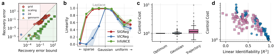
Figure 4 解读：四个 panel 对应四个主结论的实验支持。a) approximate bound verification：grid、2D、scaling、gennorm runs 大多落在 diagonal 以下，说明 theorem 3 的 bound 没被破坏；b) Gaussian optimality：当 generalized-normal shape $\alpha =2$（Gaussian）时 $R^2(h\to z)$ peak，偏离 Gaussian 后恢复质量下降；c) control cost：Gaussian encoder 与 oracle 统计上不可区分，trajectory encoder 偏高；d) control cost 随 linear identifiability $R^2$ 单调下降，支持 theorem 4。

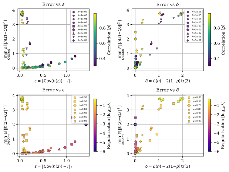
Figure 6/Appendix bound decomposition 解读：左列把 recovery error 对 $\epsilon$（whitening deviation）作图，右列对 $\delta$（alignment gap）作图。结果显示 $\delta$ 比 $\epsilon$ 更能预测 recovery error；$\lambda =0.5$ 的 run 甚至能把 $\epsilon$ 做得很小，但因为 alignment 信号被压制，表示仍会崩掉。这与 theorem 3 的解释一致：approximate whitening 是容易部分，binding constraint 是 alignment quality。

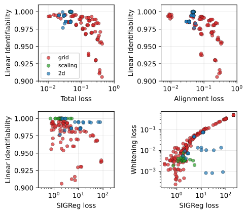
Appendix loss-predictivity figure 解读：scatter plots 把 training losses 与 linear identifiability 联系起来，说明不是所有低 regularization loss 都代表好 World Model；只有 alignment gap 足够小且 distribution constraint 不主导训练时，$h$ 才接近 rotation of $z$。

5.4 Generalized-normal ablation：Gaussian 是 sharp optimum

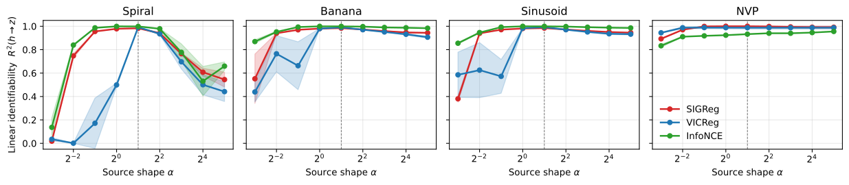
Figure 7 解读：横轴是 generalized-normal shape $\alpha$，其中 $\alpha =1$ 是 Laplace，$\alpha =2$ 是 Gaussian。四个 2D mixing 上，linear identifiability $R^2(h\to z)$ 都在 $\alpha =2$ 附近达到峰值，偏离 Gaussian 后下降；这直接展示 theorem 2 的 empirical footprint。

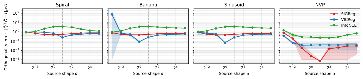
Appendix generalized-normal orthogonality 解读：orthogonality error 与 $R^2$ 互补：Gaussian 附近拟合出的线性 map 更接近 orthogonal，非 Gaussian tails 或 near-uniform source 会让 learned representation 产生不可忽略的 distortion。

5.5 Grid search：alignment 与 Gaussianity 的平衡

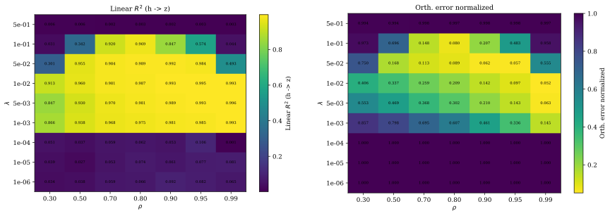
Figure 6 解读：左图是 $R^2$，右图是 normalized orthogonality error；横轴扫 $\rho$，纵轴扫 SIGReg weight $\lambda$。太强的 Gaussianity（例如 $\lambda =0.5$）会让 SIGReg 主导而损害 alignment，导致 collapse / poor recovery；在 alignment signal 足够强时，较小 $\lambda$ 就能维持 Gaussianity 并恢复 latent。这个图说明 LeJEPA 的理论 guarantee 不等价于“SIGReg 越强越好”，而是要让 Gaussian constraint 与 positive-pair alignment 同时有效。

5.6 Pixel-based Reacher：真实渲染观测下的 planning 证据

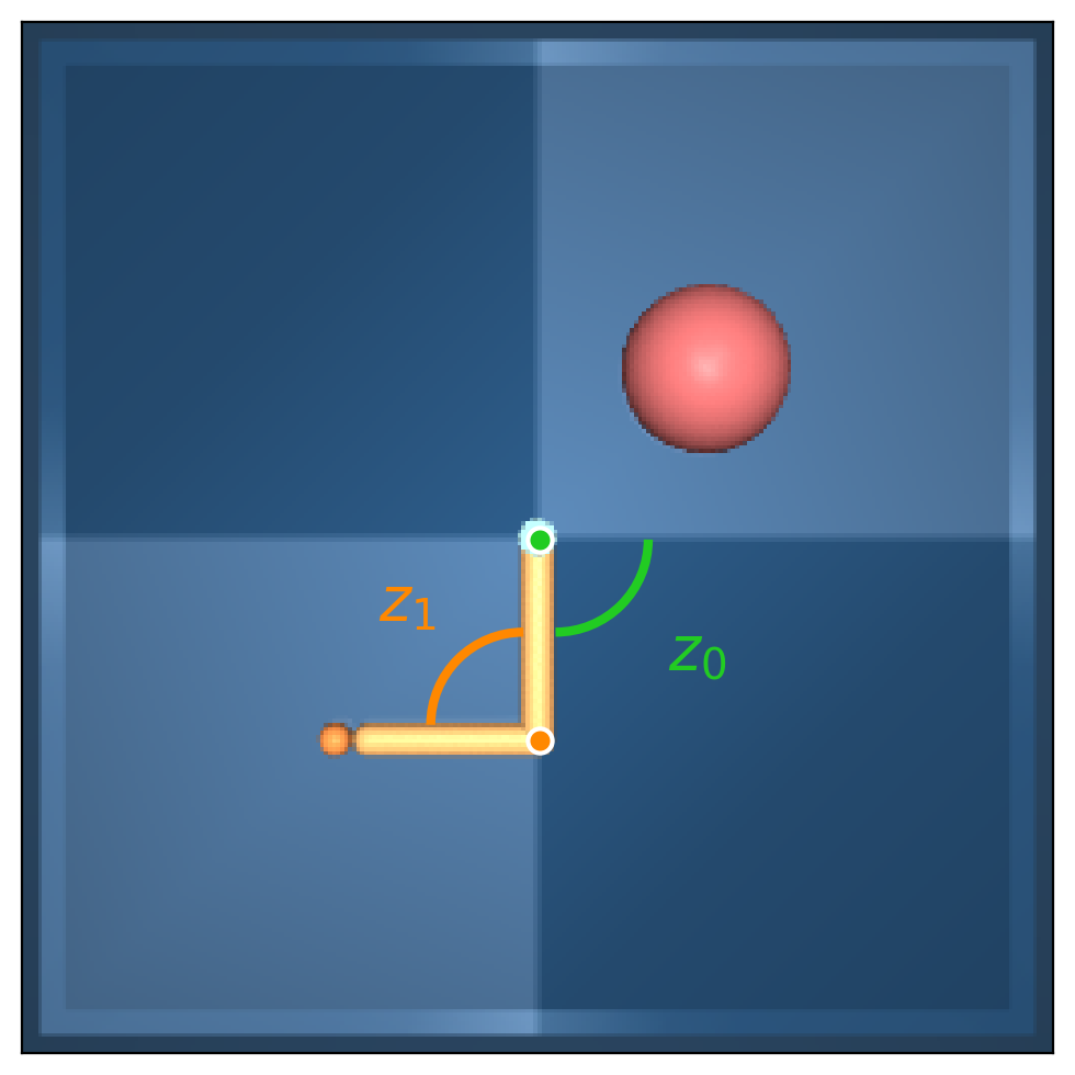
Appendix Reacher figure 解读：Reacher 的真实 latent 是两个 joint angles，MuJoCo rendering pipeline 是复杂非线性 $g$，生成 $64\times 64$ RGB observation。这是从低维 synthetic mixing 走向 pixel observation 的关键实验：如果 LeJEPA 能在像素上恢复 joint-angle latent，planning claim 才更有说服力。

Main text Table 2 报告 OU Gaussian pairs 与 RL-policy trajectories 的对比：

OU $\rho$	OU $R^2(z\to h)$	OU $R^2(h\to z)$	Traj stride $\delta$	${\rho }_0$	${\rho }_1$	Traj $R^2(z\to h)$	Traj $R^2(h\to z_0)$	Traj $R^2(h\to z_1)$
0.30	0.67 ± 2e-02	0.67 ± 2e-02	1	1.000	0.999	-0.39 ± 1e-01	0.71 ± 3e-02	-0.03 ± 4e-02
0.50	0.86 ± 1e-02	0.86 ± 1e-02	2	0.999	0.996	-0.47 ± 5e-02	0.73 ± 4e-03	0.01 ± 2e-03
0.70	0.93 ± 7e-03	0.93 ± 7e-03	4	0.997	0.991	-0.05 ± 3e-01	0.51 ± 1e-01	0.43 ± 9e-02
0.80	0.94 ± 3e-04	0.94 ± 3e-04	8	0.992	0.982	0.50 ± 2e-02	0.80 ± 2e-03	0.78 ± 6e-03
0.90	0.95 ± 7e-04	0.95 ± 7e-04	16	0.981	0.963	0.44 ± 4e-02	0.63 ± 2e-02	0.87 ± 2e-02
0.95	0.95 ± 2e-04	0.95 ± 2e-04	32	0.959	0.928	0.45 ± 6e-02	0.62 ± 2e-02	0.81 ± 1e-02
0.99	0.95 ± 4e-04	0.95 ± 4e-04	64	0.915	0.863	0.44 ± 4e-02	0.55 ± 3e-02	0.77 ± 2e-02

OU condition 随 $\rho$ 增大达到约 $R^2=0.95$，说明满足 Gaussian + isotropic OU assumptions 时，pixel encoder 也能恢复 joint-angle latent。trajectory condition 则出现 anisotropy（${\rho }_0\ne {\rho }_1$）和非 Gaussian transition，导致总 $R^2$ 明显较低；有些 stride 下某个 joint 可以被恢复，但整体 representation 不再是 clean orthogonal map。

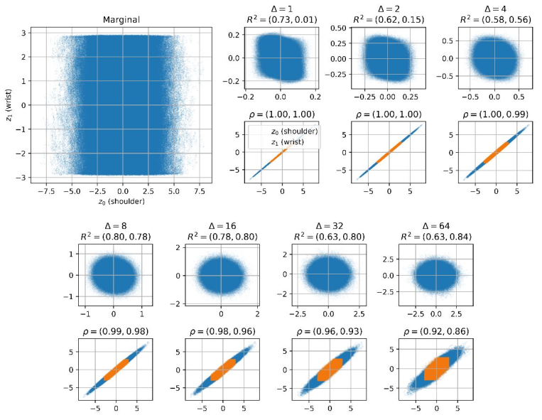
Appendix Reacher distribution figure 解读：trajectory samples 的 latent distribution 沿 policy-induced manifold 收缩，不像 OU samples 那样 isotropic 覆盖 joint space。这解释了为什么同一个物理系统在 OU sampling 下可识别，在 goal-directed policy trajectories 下不可识别：数据分布本身已经违反 theorem assumptions。

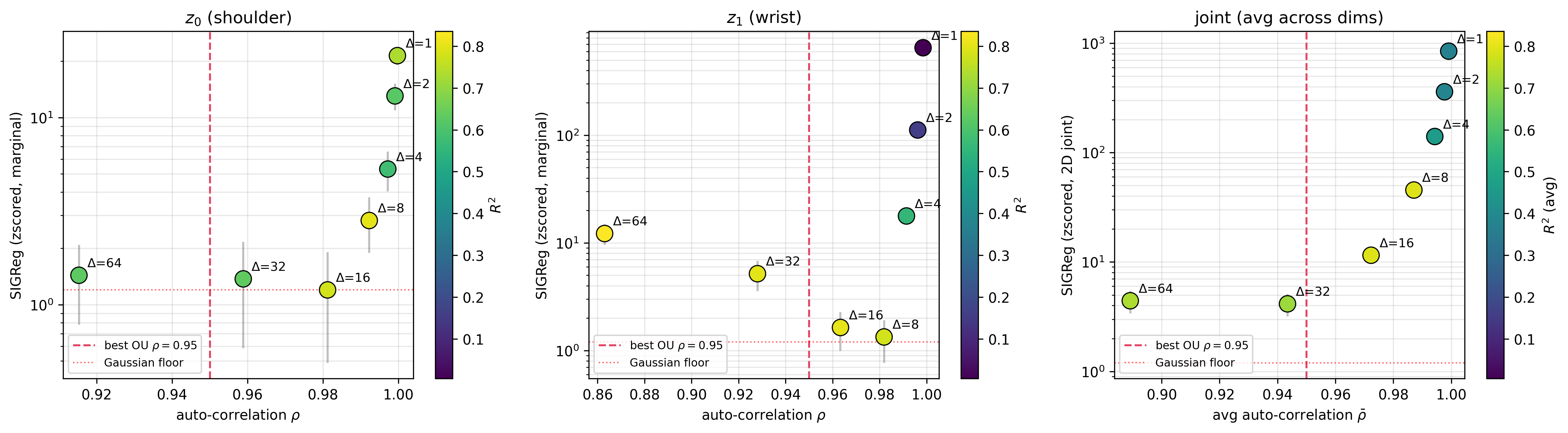
Appendix Reacher $\rho$ / SIGReg figure 解读：identifiability 需要两个条件同时成立：positive pairs 不能完全无关，embedding distribution 也不能失去 Gaussianity。低 $\rho$ alignment signal 太弱，高偏置 trajectory distribution 又破坏 isotropy。

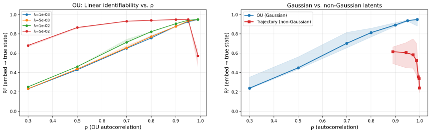
Appendix Reacher R2 group 解读：左侧 OU sweep 显示 $R^2$ 随 $\rho$ 增加而上升；右侧 OU vs trajectory 对比显示，policy trajectory 即使 temporal correlation 高，也因为覆盖低熵区域和各维相关性不均衡，无法得到同样的 linear recovery。

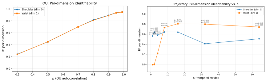
Appendix per-dimension R2 group 解读：OU condition 的两个 latent dimensions 都能被较均衡地恢复；trajectory condition 则出现 per-dimension asymmetry，说明 representation 不是整体 orthogonal rotation，而是偏向恢复 policy 经常访问或变化更显著的自由度。

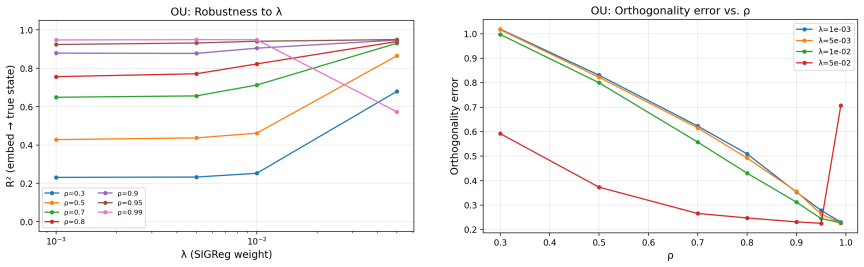
Appendix lambda / orthogonality group 解读：$\lambda$ 的鲁棒性图与 grid-search 结论一致：regularization 过弱无法维持 Gaussianity，过强会牺牲 alignment；orthogonality error 则提供比 $R^2$ 更细的几何质量诊断。

5.7 Latent-space planning：只有 identifiable encoder 的 straight line 仍是 straight line

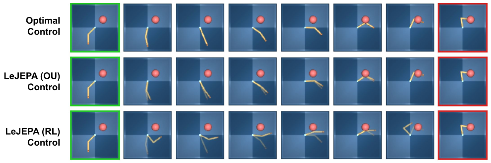
Figure 5 解读：top 是 oracle joint-space straight-line control；middle 是 Gaussian-OU encoder 的 latent interpolation，decode 后几乎贴合 oracle；bottom 是 RL-trajectory encoder，同样做 latent interpolation 却产生明显偏离。这个 qualitative result 连接 theorem 4：linear identifiability 不是只为了 probe 好看，而是直接决定 latent-space planning 是否保真。

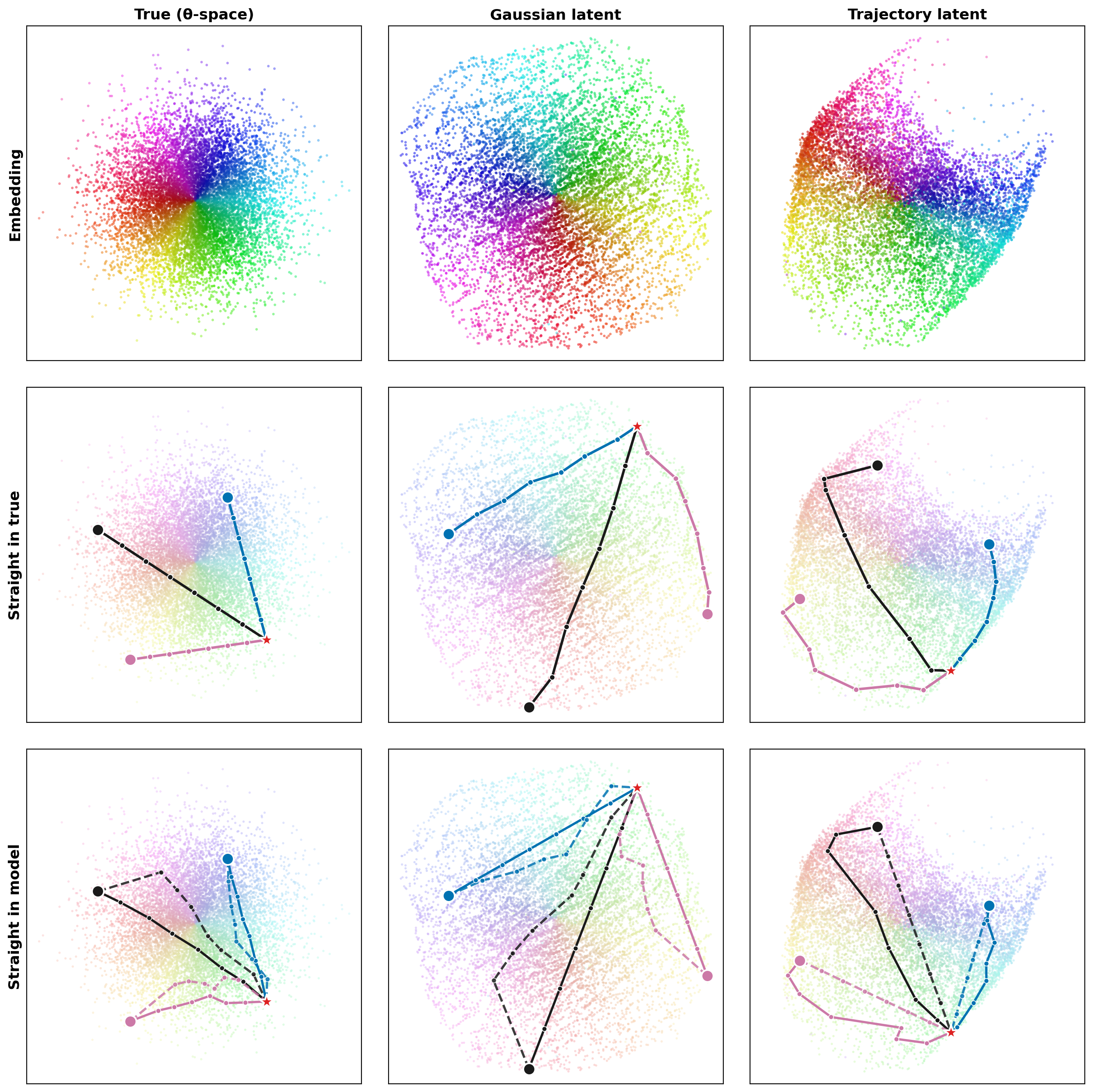
Appendix planning scatter 解读：左列是真实 $\theta$-space，中列是 Gaussian/OU encoder，右列是 trajectory encoder。top row 显示 embedding geometry，middle/bottom row 分别测试 true-space straight lines 和 latent-space straight lines。Gaussian encoder 近似 rotation，因此两种 straightness 互相保持；trajectory encoder 明显 warped，latent straight line decode 回真实空间后弯曲。

5.8 Overall conclusions and Limitations

实验总体支持四个结论：

1. 在 Gaussian OU world 中，LeJEPA/SIGReg 能把 nonlinear observation 恢复成与 true latent 线性等价的表示。
2. Gaussian assumption 是 sharp 的：generalized-normal sweep 在 $\alpha =2$ 处达到峰值，偏离 Gaussian 后 identifiability 下降。
3. Approximate theorem 的主导误差是 alignment gap $\delta$，而不是单独的 covariance / whitening error $\epsilon$。
4. Linear identifiability 与 planning quality 直接相关；在 Reacher 中，Gaussian-OU encoder 的 latent planning 接近 oracle，trajectory encoder 则偏离。

作者明确承认的限制包括：真实世界 latent 是否 Gaussian 无法仅从 observations 判断；theorem 假设 encoder output dimension $m$ 等于 true latent dimension $n$，当 $m<n$ 或 $m>n$ 时会涉及 subspace selection、superposition 或 redundancy；理论是 population-level global optimum，虽然有 approximate bound，但未给出 finite-sample scaling 或 optimization dynamics guarantee；此外本文证明的是 state representation 的 identifiability，action-conditioned dynamics $\hat{p}({\hat{z}}^{\prime }\mid \hat{z},a)$ 仍需要额外学习。