Revisiting Feature Prediction for Learning Visual Representations from Video

Paper: arXiv:2404.08471 Code: facebookresearch/jepa Code reference: main @ 51c59d51 (2025-02-27)

1. Motivation (研究动机)

这篇论文要回答的问题很直接：只靠视频里的 feature prediction，能不能训练出通用视觉表征？ 这里的“只靠”是重点。作者明确排除了 pretrained image encoder、text、negative examples、pixel-level reconstruction、human annotations 等额外监督或辅助目标，只保留一个 Joint-Embedding Predictive Architecture (JEPA) 式的 latent feature prediction 目标。这个设定之所以重要，是因为过去很多 video representation learning 方法虽然也谈“预测未来”或“预测缺失区域”，但常常依赖额外机制来防止 collapse：例如 contrastive negatives、冻结好的 image/video encoder、action forecasting supervision，或者直接重建 pixel。这样得到的结果很难说明“预测 representation 本身”是否足够。

现有方法的第一个瓶颈是 pixel reconstruction 把大量容量花在低层细节上。VideoMAE / masked autoencoding 一类方法需要还原像素，因此模型必须解释纹理、颜色、局部噪声和不可预测细节；这些细节对 downstream action recognition、motion understanding 或 object-centric semantics 不一定有用。论文认为 latent feature space 的目标更灵活：目标 encoder 可以把不可预测或无关的 pixel-level variation 压缩掉，predictor 只需要预测对语义、运动和时空一致性有用的表示。

第二个瓶颈是 视频任务同时需要 appearance 与 motion。Kinetics-400 的很多类别只看物体或场景就能猜到，偏 appearance；Something-Something-v2 则刻意削弱物体外观与动作标签的关联，更依赖细粒度时序与物体运动。一个好的 frozen video backbone 不应只在其中一类任务上强，而应该能在同一组参数下同时支持 appearance-heavy 和 motion-heavy downstream tasks。

第三个瓶颈是 训练效率与样本效率。论文将 V-JEPA 与 OpenCLIP、DINOv2、VideoMAEv2 等大规模模型对比时强调，V-JEPA 的 ViT-H/16 $_{384}$ 只处理约 210M video clips，而 OpenCLIP / DINOv2 / VideoMAEv2 对应表中的样本数是 39000M / 1900M / 1600M。即使不同数据模态和训练协议不能完全等价，这也说明作者关心的不是单纯堆数据，而是探索 feature prediction 作为 pretraining objective 的效率。

因此，这篇论文的目标可以概括为：构造一个现代化的 video JEPA 训练方案，在 2M public videos 组成的 VideoMix2M 上从头训练 ViT-L/16、ViT-H/16 和 ViT-H/16 $_{384}$ ，然后用 frozen backbone + lightweight attentive probe 以及 full fine-tuning 两种协议检验表征是否真正通用。若成立，它支持 Yann LeCun 所倡导的 JEPA/world-model 路线中的一个核心命题：智能系统可以通过预测抽象表征来学习世界的结构，而不必在像素空间复原每个细节。

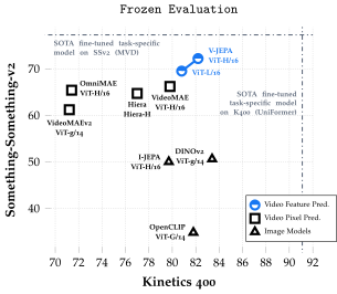
Figure 1 解读：横轴/纵轴对应 Kinetics-400 与 Something-Something-v2 等视频任务上的 frozen evaluation 表现。V-JEPA 的位置说明它不是只学到 object/scene appearance，也能保留 motion-sensitive information。作者用这张图强调：同一个 frozen backbone 能同时迁移到 appearance-heavy 与 motion-heavy 任务，这是 feature prediction 是否“通用”的关键证据。

2. Idea (核心思想)

核心 insight 是：不要预测像素，而是在一个由 EMA target encoder 产生的 latent feature space 中预测被 mask 的视频区域；同时用大比例、连续的 3D multi-block masks 迫使模型利用时空上下文，而不是抄局部纹理。这个目标把学习压力从“重建可见外观细节”转移到“在抽象表示中补全缺失的时空语义”。

V-JEPA 的创新不在于提出一个全新的 Transformer block，而在于把三个设计组合成一个可独立工作的 video self-supervised objective：1）Joint-Embedding Predictive Architecture，用 x-encoder + predictor 预测 y-encoder 的表示；2）EMA target encoder + stop-gradient 防止表征塌缩；3）短程/长程 multi-block masking，使预测任务同时覆盖局部缺失和大范围缺失。与 VideoMAE 的根本差别是预测目标：VideoMAE 回到 pixels，V-JEPA 回到 target encoder features；与 contrastive video methods 的差别是训练不需要 negative clips，也不把远处视频片段当作负例。

从 world-model 角度看，V-JEPA 学的是“可预测的 latent state”，不是 pixel generator。论文后续用 conditional diffusion decoder 只是为了离线可视化 predicted features 中包含的信息；V-JEPA 本体在训练和下游评估中都没有 pixel decoder。

3. Method (方法)

3.1 Overall framework：从 JEPA 到 V-JEPA

JEPA 的一般形式是：给定一个输入区域 $x$ 、目标区域 $y$ 和描述二者关系的条件变量 $z \leftarrow Δ_{y}$ ，encoder $E_{θ}$ 先把 $x$ 编成 representation，predictor $P_{ϕ}$ 再根据 $z$ 预测 $y$ 的 representation。朴素目标为： $min_{θ, ϕ} ∥ P_{ϕ} (E_{θ} (x), Δ_{y}) - E_{θ} (y) ∥_{1} .$ 这个目标有 trivial constant solution：如果 encoder 对任何输入都输出常数，loss 也可以很小。V-JEPA 采用 BYOL / I-JEPA 风格的 collapse prevention，把 target side 改成 stop-gradient + EMA encoder： $min_{θ, ϕ} P_{ϕ} (E_{θ} (x), Δ_{y}) - sg (\overline{E}_{θ} (y))_{1},$ 其中 $sg (\cdot)$ 表示不反传梯度， $\overline{E}_{θ}$ 是 online encoder $E_{θ}$ 的 exponential moving average。直觉上，predictor 总是在追一个较慢移动的 target representation；如果 predictor 近似最优， $ℓ_{1}$ 目标对应条件中位数 $median (Y ∣ E_{θ} (x))$ ，encoder 为了降低 conditional median absolute deviation 必须保留更多与目标区域相关的信息，而不是任意塌缩。

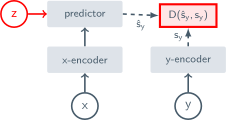
Figure 2 解读：普通 JEPA 把学习问题写成“从 $x$ 的 representation 预测 $y$ 的 representation”。变量 $z$ 告诉 predictor 当前要预测的目标位置或变换类型。在 V-JEPA 中， $z$ 具体化为 masked spatio-temporal patches 的 3D positional embedding；这让同一个 context representation 能针对不同缺失区域产生不同预测。

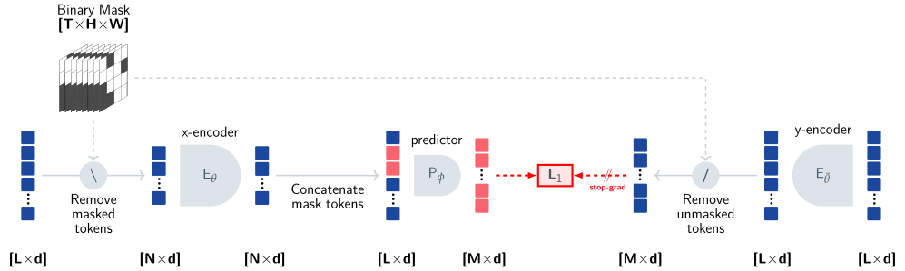
Figure 3 解读：V-JEPA 的训练链路从左到右是：把 $T$ 帧视频 patchify 成 spatio-temporal token 序列；对 context 侧直接 drop 掉被 mask 的 token；x-encoder 只处理剩余 token；predictor 把 x-encoder 输出与带 3D 位置的 learnable mask tokens 拼接；最后只对 target tokens 的 predictor 输出与 y-encoder 输出做 $L_{1}$ regression。这里的关键是 x-encoder 不看到被 mask 的 patch，y-encoder 看到完整 clip 但通过 stop-gradient/EMA 只提供目标。

3.2 视频 tokenization 与 3D patch 表示

V-JEPA 使用 Vision Transformer 作为 video backbone。输入 clip 有 16 frames，相邻帧 temporal stride 为 4。每个 token 对应一个 $16 \times 16 \times 2$ 的 spatio-temporal tubelet；因此在 $224 \times 224$ 分辨率下，token 数为 $(16/2) \times (224/16)^{2} = 8 \times 14 \times 14 = 1568$ ，论文在 appendix 中记为 $L = 1568$ 。对于 $384 \times 384$ 输入，空间 grid 变为 $24 \times 24$ ，token 数更大，但训练逻辑相同。

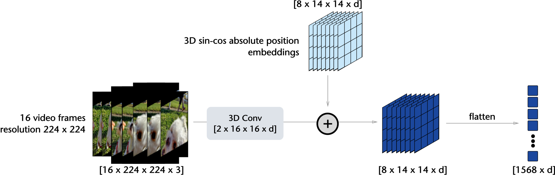
Figure 7 解读：这张图展示了 V-JEPA 如何把视频切成 3D patches。与 image MAE 的 2D patch 不同，每个 token 跨两个连续 frames，因此 token 自带短时运动线索。后续 mask 与 predictor 都在这个 spatio-temporal token grid 上工作，而不是在 raw pixel grid 上逐点建模。

3.3 Multi-block masking：预测什么、从什么预测

论文的 prediction task 采用 masked modeling formulation。目标区域 $y$ 是若干空间连续 block 的 union，这些 block 会沿整个 temporal dimension 重复；context $x$ 是其 complement。作者强调大块连续 mask 能降低信息泄漏，因为视频存在强空间/时间冗余，如果只随机丢少量 token，模型可能通过邻近 patch 的低层纹理插值解决任务，而不必学习抽象运动和物体状态。

默认 V-JEPA 使用两类 masks：

short-range masks：采样 8 个 target blocks，每个 block spatial scale 为 0.15；
long-range masks：采样 2 个 target blocks，每个 block spatial scale 为 0.7；
两者 aspect ratio 都在 $(0.75, 1.5)$ 中随机采样，temporal scale 为 1.0，即 mask 延伸到整个 clip 的时间轴；平均 masking ratio 约为 $90%$ 。

released code 中的 configs/pretrain/vitl16.yaml、configs/pretrain/vith16.yaml、configs/pretrain/vith16_384.yaml 对应两个 mask entries：第一个 num_blocks=8, spatial_scale=[0.15,0.15], temporal_scale=[1.0,1.0]，第二个 num_blocks=2, spatial_scale=[0.7,0.7], temporal_scale=[1.0,1.0]。src/masks/multiblock3d.py 的 MaskCollator 为每个 batch 产生 masks_enc 与 masks_pred：先在 3D grid 上把 target block 置 0，mask_p 收集 target indices，mask_e 收集 complement context indices；为了 batch 内形状一致，会截断到当前 batch 的最小 keep 数。

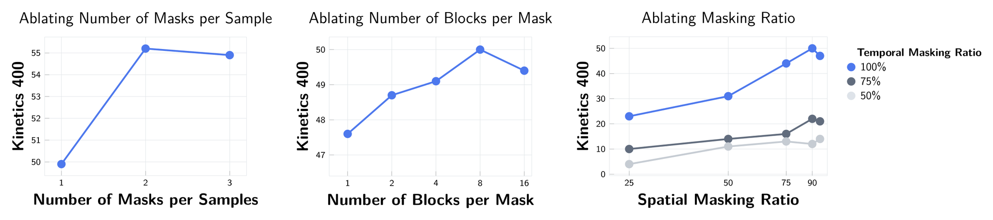
Figure 8a–8c 解读：appendix 的 masking ablation 显示三件事：每个 clip 采样多个 masks 有收益；固定高 mask ratio 时，block 数量会影响任务难度；spatial/temporal masking ratio 都需要足够高。特别是 temporal ratio 为 100% 时，空间 mask 会贯穿所有 frames，迫使模型基于可见区域的时空结构推断被遮挡对象，而不是利用相邻帧泄漏。

Figure 9a–9c 解读：这组 mask visualization 对应不同 block 数和 block size。block 越少、单块越大，模型越难通过局部纹理插值恢复目标；block 越多、单块越小，则更像随机遮挡。V-JEPA 的默认 short/long mask 组合试图同时覆盖局部细节补全和大范围语义补全。

3.4 V-JEPA loss 的逐步定义

论文 appendix 把一个训练 step 写得更具体。记完整视频 token 序列为 $x_{L} = (x_{1}, \dots, x_{L})$ 。给定 masked indices $(i_{1}, \dots, i_{M})$ 与 unmasked indices $(j_{1}, \dots, j_{N})$ ，context clip 为： $x_{N} = (x_{j_{1}}, \dots, x_{j_{N}}) .$ x-encoder 输出 context representations： $z_{N} = E_{θ} (x_{N}) = (z_{j_{1}}, \dots, z_{j_{N}}) .$ predictor 使用 context tokens 与 target mask tokens $m_{M} = (m_{i_{1}}, \dots, m_{i_{M}})$ ，输出 masked positions 的预测： $\overset{s}{^}_{M} = P_{ϕ} (z_{N}, m_{M}) = (\overset{s}{^}_{i_{1}}, \dots, \overset{s}{^}_{i_{M}}) .$ y-encoder 处理完整 unmasked video clip 得到 target representations： $s_{L} = \overline{E}_{θ} (x_{L}) = (s_{1}, \dots, s_{L}) .$ 最终 loss 是 masked target positions 上的平均 $L_{1}$ distance： $L = \frac{1}{M} \sum_{k \in (i_{1}, \dots, i_{M})} ∥ \overset{s}{^}_{k} - s_{k} ∥_{1} .$ released code 中 app/vjepa/train.py 的 loss_fn 实现为 torch.mean(torch.abs(zi-hi)**loss_exp)/loss_exp，默认 config 里 loss_exp=1.0，因此等价于 mean absolute error；当有 short-range 与 long-range 两组 masks 时，code 会对每组 mask 的 loss 求和后除以 len(masks_pred)。

3.5 Predictor 与 target encoder 的实现细节

src/models/predictor.py 的 VisionTransformerPredictor 先用 linear layer 把 context encoder 的 embedding 映射到 pred_embed_dim=384。当 use_mask_tokens=true（released pretrain configs 均为 true）时，target side 不直接使用 target features 输入 predictor，而是取一个 learnable mask_token，repeat 到全 patch grid，再用 masks_tgt 选出 masked positions；随后加上 3D sin-cos positional embedding。最后 code 将 context tokens 与 target prediction tokens concat，经过 predictor_blocks，取输出序列中 target token 部分，再通过 predictor_proj 投回 encoder feature dimension。

这与论文图示一致：predictor 的输入包含 context representation 和“我要预测哪些位置”的 mask tokens；target encoder 的 features 只作为 loss target。值得注意的是 code 的 predictor API 仍接收 tgt 参数，因为它也支持 mask_tokens is None 时对 target features 做 diffusion/noise 的分支；但 V-JEPA 论文对应的 released configs 使用 mask tokens，因此该分支不是本文主实验路径。

训练时，target_encoder 是 online encoder 的拷贝并设为 requires_grad=False；每次 optimizer step 后执行 EMA update： $\overset{ˉ}{θ} \leftarrow m \overset{ˉ}{θ} + (1 - m) θ,$ 其中 released config 的 ema 从 0.998 schedule 到 1.0。这让 target representation 慢于 online encoder，配合 stop-gradient 防止 collapse。

论文公式与 released code 实现差异：未发现会改变核心目标的冲突。 主要实现层面的差异/补充是：论文公式写成单个 mask 的 $\frac{1}{M} \sum ∥ \overset{s}{^}_{k} - s_{k} ∥_{1}$ ，released code 同时跑 short-range 与 long-range 两个 mask configs，并对两组 prediction losses 取平均；论文文字强调 learnable mask tokens + 3D positional embedding，code 中也如此，但 predictor 函数保留了一个 unused-in-config 的 target-feature diffusion 分支。

3.6 Source-grounded pseudocode

下面伪代码按 released repo facebookresearch/jepa 的 main@51c59d51 归纳，不是论文文字的抽象复述。

import torch
import torch.nn.functional as F
 
 
def sample_multiblock_masks(batch_size, grid_t, grid_h, grid_w, cfg):
    """Based on src/masks/multiblock3d.py::MaskCollator/_MaskGenerator."""
    pred_masks, enc_masks = [], []
    min_pred, min_enc = grid_t * grid_h * grid_w, grid_t * grid_h * grid_w
    block_size = sample_block_size(
        temporal_scale=cfg["temporal_scale"],
        spatial_scale=cfg["spatial_scale"],
        aspect_ratio=cfg["aspect_ratio"],
    )
    for _ in range(batch_size):
        context_empty = True
        while context_empty:
            keep = torch.ones(grid_t, grid_h, grid_w, dtype=torch.int32)
            for _ in range(cfg["num_blocks"]):
                block = sample_3d_block_mask(block_size, grid_t, grid_h, grid_w)
                keep *= block                      # block has 0 on target positions
            target_idx = torch.argwhere(keep.flatten() == 0).squeeze()
            context_idx = torch.nonzero(keep.flatten()).squeeze()
            context_empty = len(context_idx) == 0
        min_pred = min(min_pred, len(target_idx))
        min_enc = min(min_enc, len(context_idx))
        pred_masks.append(target_idx)
        enc_masks.append(context_idx)
    pred_masks = torch.stack([m[:min_pred] for m in pred_masks])
    enc_masks = torch.stack([m[:min_enc] for m in enc_masks])
    return enc_masks, pred_masks

class VJEPAPredictor(torch.nn.Module):
    """Based on src/models/predictor.py::VisionTransformerPredictor.forward."""
    def forward(self, ctxt, tgt, masks_ctxt, masks_tgt, mask_index=1):
        B = len(ctxt) // len(masks_ctxt)
        x = self.predictor_embed(ctxt)
        x = x + apply_masks(self.pos_embed.repeat(B, 1, 1), masks_ctxt)
 
        if self.mask_tokens is not None:
            pred = self.mask_tokens[mask_index % self.num_mask_tokens]
            pred = pred.repeat(B, self.num_patches, 1)
            pred = apply_masks(pred, masks_tgt)
        else:
            pred = self.diffusion(self.predictor_embed(tgt))
 
        pos = apply_masks(self.pos_embed.repeat(B, 1, 1), masks_tgt)
        pos = repeat_interleave_batch(pos, B, repeat=len(masks_ctxt))
        pred = pred + pos
 
        x = x.repeat(len(masks_tgt), 1, 1)
        x = torch.cat([x, pred], dim=1)
        masks = torch.cat([torch.cat(masks_ctxt, dim=0), torch.cat(masks_tgt, dim=0)], dim=1)
        for blk in self.predictor_blocks:
            x = blk(x, mask=masks)
        x = self.predictor_norm(x)
        return self.predictor_proj(x[:, ctxt.shape[1]:])

 
def vjepa_train_step(clips, masks_enc, masks_pred, encoder, target_encoder, predictor, optimizer, momentum):
    """Based on app/vjepa/train.py::train_step with loss_exp=1.0."""
    with torch.no_grad():
        h = target_encoder(clips)
        h = F.layer_norm(h, (h.size(-1),))
        h = apply_masks(h, masks_pred, concat=False)
 
    z_context = encoder(clips, masks_enc)
    z_pred = predictor(z_context, h, masks_enc, masks_pred)
 
    loss = 0.0
    for z_i, h_i in zip(z_pred, h):
        loss = loss + torch.mean(torch.abs(z_i - h_i))
    loss = loss / len(masks_pred)
 
    optimizer.zero_grad(set_to_none=True)
    loss.backward()
    optimizer.step()
 
    with torch.no_grad():
        for online, target in zip(encoder.parameters(), target_encoder.parameters()):
            target.data.mul_(momentum).add_((1.0 - momentum) * online.detach().data)
    return loss

class FrozenAttentiveProbe(torch.nn.Module):
    """Based on src/models/attentive_pooler.py and appendix frozen evaluation."""
    def __init__(self, embed_dim, num_classes):
        super().__init__()
        self.query = torch.nn.Parameter(torch.zeros(1, 1, embed_dim))
        self.cross_attention = CrossAttentionBlock(dim=embed_dim, num_heads=embed_dim // 64)
        self.classifier = torch.nn.Linear(embed_dim, num_classes)
 
    def forward(self, frozen_tokens):
        q = self.query.expand(frozen_tokens.size(0), -1, -1)
        pooled = self.cross_attention(q, frozen_tokens)
        return self.classifier(pooled[:, 0])

Code reference: main @ 51c59d51 (2025-02-27) — pseudocode and mapping based on this commit

Paper Concept	Source File	Key Class/Function
V-JEPA pretraining loop, target encoder, loss, EMA update	`app/vjepa/train.py`	`train_step`, `forward_target`, `forward_context`, `loss_fn`
3D multi-block masking for short/long range masks	`src/masks/multiblock3d.py`	`MaskCollator`, `_MaskGenerator.__call__`, `_sample_block_mask`
Predictor with learnable mask tokens and 3D positional embeddings	`src/models/predictor.py`	`VisionTransformerPredictor.forward`
Video/image ViT tokenization and masked token dropping	`src/models/vision_transformer.py`	`VisionTransformer.forward`, `PatchEmbed3D`
Frozen attentive probing	`src/models/attentive_pooler.py`; `evals/video_classification_frozen/eval.py`; `evals/image_classification_frozen/eval.py`	`AttentivePooler`, frozen eval loops
Actual pretraining configs used for numbers	`configs/pretrain/vitl16.yaml`; `configs/pretrain/vith16.yaml`; `configs/pretrain/vith16_384.yaml`	`data`, `mask`, `model`, `optimization` sections
Actual frozen evaluation configs	`configs/evals/vith16_384_k400_16x8x3.yaml`; `configs/evals/vith16_384_ssv2_16x2x3.yaml`; image eval YAMLs	dataset classes, views/clips, probe LR/epochs

4. Experimental Setup (实验设置)

Pretraining datasets and scale

V-JEPA 的主预训练数据是 VideoMix2M，由公开视频数据合并并去重验证集重叠得到：HowTo100M (HT)、Kinetics-400/600/700 合并记作 K710，以及 Something-Something-v2 (SSv2)。论文明确报告的 pretraining data distribution 为：K710 约 700K videos，K710+SSv2 约 900K videos，K710+HT 约 1900K videos，VideoMix2M 约 2000K videos。主模型使用 VideoMix2M。

下游评估覆盖视频与图像任务：Kinetics-400 (K400, 400 classes, action recognition, appearance-heavy)、Something-Something-v2 (SSv2, 174 classes, motion classification, motion-heavy)、AVA (action localization)、ImageNet-1K (1000 classes)、Places205 (205 classes)、iNaturalist-2021 (10K classes)。论文/配置文件明确给出 class counts；逐项样本数除 pretraining distribution 和 low-shot per-class counts 外未在正文完整列出，因此这里不把公开基准的常见样本数当作作者重新统计。

Baselines

论文分三类比较：

Pixel prediction video baselines：OmniMAE、VideoMAE、Hiera，均依赖 pixel reconstruction / masked autoencoding。
Image-pretrained baselines：I-JEPA、OpenCLIP、DINOv2，用于观察强 image representation 在 video tasks 上的迁移边界。
Video/self-supervised baselines：MVD、OmniMAE、VideoMAE、VideoMAEv2、Hiera，并在 fine-tuning 表中额外比较 VideoMAEv1、VideoMAEv2、MVD。

Metrics and protocols

主要指标是 top-1 accuracy；AVA 使用 action localization 的 mAP 类指标（表中记为 AVA 分数）。评估协议有两种：

Frozen evaluation with attentive pooling：冻结 V-JEPA backbone，只训练一个 lightweight attentive probe。视频任务常用多 clip / multi-view 输入，例如 K400 的 16×8×3 表示 16 frames、8 temporal segments、3 spatial views；SSv2 使用 16×2×3。Image tasks 使用 frozen encoder + probe。
End-to-end fine-tuning：在 K400 和 SSv2 上完整 fine-tune，推理时使用 multi-view fusion，例如 K400 16×5×3、SSv2 16×2×3。

Training config from released launch configs

训练配置来自 released repo 的实际 YAML，而不是 base defaults：

`configs/pretrain/vitl16.yaml`

Model / input：model_name=vit_large，crop_size=224，num_frames=16，sampling_rate=4，patch_size=16，tubelet_size=2。
Distributed batch：nodes=16，tasks_per_node=8，per-GPU data.batch_size=24，global batch size $16 \times 8 \times 24 = 3072$ 。
Optimization：epochs=300，ipe=300，总 iterations $300 \times 300 = 90000$ ；warmup=40 epochs，即 $40 \times 300 = 12000$ iterations；start_lr=2e-4，lr=6.25e-4，final_lr=1e-6；weight_decay=0.04 到 final_weight_decay=0.4；EMA [0.998, 1.0]；dtype=bfloat16，paper table 报告 accelerator 为 A100 80G。
Masking：两个 mask configs，分别是 8 blocks / 0.15 spatial scale 与 2 blocks / 0.7 spatial scale，temporal scale 均为 1.0，aspect ratio [0.75,1.5]。

`configs/pretrain/vith16.yaml`

与 ViT-L/16 $_{224}$ 基本相同，但 model_name=vit_huge；global batch size 仍为 3072，总 iterations 仍为 90000。

`configs/pretrain/vith16_384.yaml`

Model / input：model_name=vit_huge，crop_size=384，其余 clip/tubelet 设置相同。
Distributed batch：nodes=30，tasks_per_node=8，per-GPU data.batch_size=10，global batch size $30 \times 8 \times 10 = 2400$ 。
Optimization / masks：同样 300 epochs、90000 iterations、12000 warmup iterations、LR $2 \times 1 0^{- 4} \to 6.25 \times 1 0^{- 4} \to 1 0^{- 6}$ 、EMA $0.998 \to 1.0$ ，short/long multi-block masks 与 224 模型一致。

Frozen evaluation configs 也来自 released YAML：例如 configs/evals/vith16_384_k400_16x8x3.yaml 使用 8 nodes × 8 tasks，K400 frames_per_clip=16、num_segments=8、num_views_per_segment=3、num_epochs=20、lr=0.001、weight_decay=0.01；configs/evals/vith16_384_ssv2_16x2x3.yaml 使用 SSv2 num_classes=174、2 segments、3 views、20 epochs；image eval YAMLs 对 IN1K / Places / iNat 使用 20 epochs、batch 16、LR 0.001，并读取 target_encoder checkpoint。

5. Experimental Results (实验结果)

5.1 Feature targets beat pixel targets under the same ViT-L/16 setup

Table 1 的关键对比是同样在 VideoMix2M 上训练 90K iterations、batch size 3072、multi-block prediction task：

Target	Arch.	K400 frozen	SSv2 frozen	IN1K frozen	K400 fine-tune
Pixels	ViT-L/16	68.6	66.0	73.3	85.4
Features	ViT-L/16	73.7	66.2	74.8	85.6

结论是 feature-space target 在 K400 frozen 上提升最大（+5.1），IN1K 也提升（+1.5），SSv2 与 fine-tuning 较小但仍不差。这个表支撑论文的核心主张：改预测空间本身就有效，而不是只靠更大模型或更多数据。

5.2 Pretraining data scale: average performance improves with VideoMix2M

Table 2 显示，在 90K iterations 和 batch size 3072 下，pretraining data 从 K710 到 VideoMix2M 增大后，平均性能提高：

Arch.	Data	Samples	K400	SSv2	IN1K	Avg.
ViT-L/16	K710	700K	75.8	63.2	73.7	70.9
ViT-L/16	K710+SSv2	900K	72.9	67.4	72.8	71.0
ViT-L/16	K710+HT	1900K	74.5	64.2	74.8	71.1
ViT-L/16	VideoMix2M	2000K	73.7	66.2	74.8	71.5
ViT-H/16	K710+SSv2	900K	75.7	66.8	73.7	72.0
ViT-H/16	VideoMix2M	2000K	74.0	68.5	75.9	72.8

细节上，任务最优并不总是来自最大数据：K710 对 K400 更好，K710+SSv2 对 SSv2 更好；但平均值 VideoMix2M 更强。这说明数据 mixture 对不同 downstream capabilities 有 trade-off。

5.3 Pooling matters: attentive probe is not a cosmetic detail

Table 3/appendix 对 frozen evaluation 的 pooling 做了关键消融：

Method	Arch.	K400 Linear	K400 Attentive	SSv2 Linear	SSv2 Attentive
VideoMAE	ViT-L/16	52.5	77.8	41.3	61.2
V-JEPA	ViT-L/16	56.7	80.8	50.1	69.5

正文中的 single-center-view pooling ablation 也报告 V-JEPA 从 average pooling 到 attentive pooling 在 K400 上提升 +17.3，在 SSv2 上提升 +16.1。解释是 video encoder 输出的是 dense token map，简单平均会抹掉时空定位信息；attentive probe 用 learnable query 选择 task-relevant tokens，更适合 frozen backbone evaluation。因此 V-JEPA 的 frozen performance 应被理解为“backbone + lightweight non-linear readout”的能力，而不是纯 linear probe。

5.4 Masking strategy ablation: multi-block 最强

Table 4 比较了不同“从什么预测什么”的 mask 设计，模型是 ViT-L/16，在 K710+SSv2 上预训练，用 single center view attentive probe 评估：

Masking	K400	SSv2	IN1K
random-tube[0.9]	51.5	46.4	55.6
causal multi-block[6]	61.3	49.8	66.9
causal multi-block[12]	71.9	63.6	72.2
multi-block	72.9	67.4	72.8

random-tube 虽然 mask ratio 高，但缺少连续 block 的结构；causal multi-block 只看前若干 frames，更像 forecasting，12 frames 明显好于 6 frames；full multi-block 最强，说明作者最终采用的任务不是简单 future prediction，而是从全 clip 的可见 spatio-temporal context 预测被遮挡的大块区域。

5.5 与 pixel prediction methods 的同架构比较

Table 5 控制在 ViT-L 或 Hiera-L 规模上，比较 pixel reconstruction methods 与 V-JEPA：

Method	Arch.	Samples Seen	Iter.	K400	SSv2	AVA	IN1K	Places205	iNat21	K400-ft	SSv2-ft
OmniMAE	ViT-L/16	2400M	1170K	65.6	60.6	14.4	75.1	59.8	66.1	84.0	74.2
VideoMAE	ViT-L/16	410M	400K	77.8	65.5	21.6	71.1	59.3	64.6	85.4	74.3
Hiera	Hiera-L	770M	1500K	75.5	64.2	15.8	68.9	58.5	56.9	87.3	75.1
V-JEPA	ViT-L/16	270M	90K	80.8	69.5	25.6	74.8	60.3	67.8	85.6	75.1

V-JEPA 在 frozen evaluation 中除 IN1K 略低于直接用 IN1K 训练的 OmniMAE（74.8 vs 75.1）外，其他任务均优于表中 pixel baselines；同时 Samples Seen 和 Iter. 明显更少。Fine-tuning 上 V-JEPA 与 Hiera-L 的 SSv2-ft 同为 75.1，K400-ft 不如 Hiera-L 的 87.3，但优于 VideoMAE-L 的 85.4。

5.6 与 state-of-the-art image/video models 的比较

更大范围 SOTA frozen comparison 中，V-JEPA 的三行结果为：

Method	Arch.	Params	Data	K400	SSv2	AVA	IN1K	Places205	iNat21
V-JEPA	ViT-L/16	200M	VideoMix2M	80.8	69.5	25.6	74.8	60.3	67.8
V-JEPA	ViT-H/16	630M	VideoMix2M	82.0	71.4	25.8	75.9	61.7	67.9
V-JEPA	ViT-H/16 $_{384}$	630M	VideoMix2M	81.9	72.2	25.0	77.4	62.8	72.6

注意 abstract 中的 “77.9% on ImageNet1K” 对应作者进一步说明的 two-layer attentive probe；SOTA table 中一层 attentive probe 的 IN1K 是 77.4。与 image-pretrained models 相比，DINOv2 在 K400/IN1K/iNat21 等 appearance/image-heavy 任务上仍强（例如 K400 83.4、IN1K 86.2、iNat21 88.8），但在 SSv2 上只有 50.6；V-JEPA-H/16 $_{384}$ 在 SSv2 达到 72.2，显示 video feature prediction 对 motion understanding 的优势。

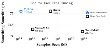
Figure 4 解读：SSv2 fine-tuning performance vs. samples seen 展示了 V-JEPA 在处理更少 pretraining clips 时达到有竞争力的 SSv2 fine-tuning 结果。它不是绝对所有任务都 SOTA，但在 motion-heavy SSv2 上，latent feature prediction 的样本效率非常突出。

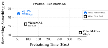
Figure 5 解读：SSv2 frozen evaluation vs. pretraining time 强调同一个结论的另一个维度：V-JEPA 在 frozen backbone 协议下以更短训练时间达到更高 motion classification 表现。这里 frozen protocol 很关键，因为它更直接反映 backbone 表征质量，而不是 fine-tuning 后网络重新适应任务的能力。

5.7 Low-shot 与 temporal coverage

Low-shot frozen evaluation 中，V-JEPA 在标注很少时优势更明显：

Method	Arch.	K400 5%	K400 10%	K400 50%	SSv2 5%	SSv2 10%	SSv2 50%
MVD	ViT-L/16	62.6±0.2	68.3±0.2	77.2±0.3	42.9±0.8	49.5±0.6	61.0±0.2
VideoMAE	ViT-H/16	62.3±0.3	68.5±0.2	78.2±0.1	41.4±0.8	48.1±0.2	60.5±0.4
VideoMAEv2	ViT-g/14	37.0±0.3	48.8±0.4	67.8±0.1	28.0±1.0	37.3±0.3	54.0±0.3
V-JEPA	ViT-H/16	67.0±0.2	72.1±0.1	80.2±0.2	51.9±0.3	57.5±0.4	67.3±0.2
V-JEPA	ViT-H/16 $_{384}$	68.2±0.2	72.8±0.2	80.6±0.2	54.0±0.2	59.3±0.5	67.9±0.2

Temporal coverage ablation 表明 K400 上把 attentive probe 从 1 clip 扩到 8 clips 能显著提升：VideoMAE-L 从 69.4 到 77.8，V-JEPA-L 从 73.7 到 80.9。V-JEPA 也受益于更长 temporal coverage，这进一步说明 frozen token map 中确实保留了跨片段有用的信息。

5.8 Qualitative visualization：V-JEPA 不是生成模型，但 predicted features 有时空一致性

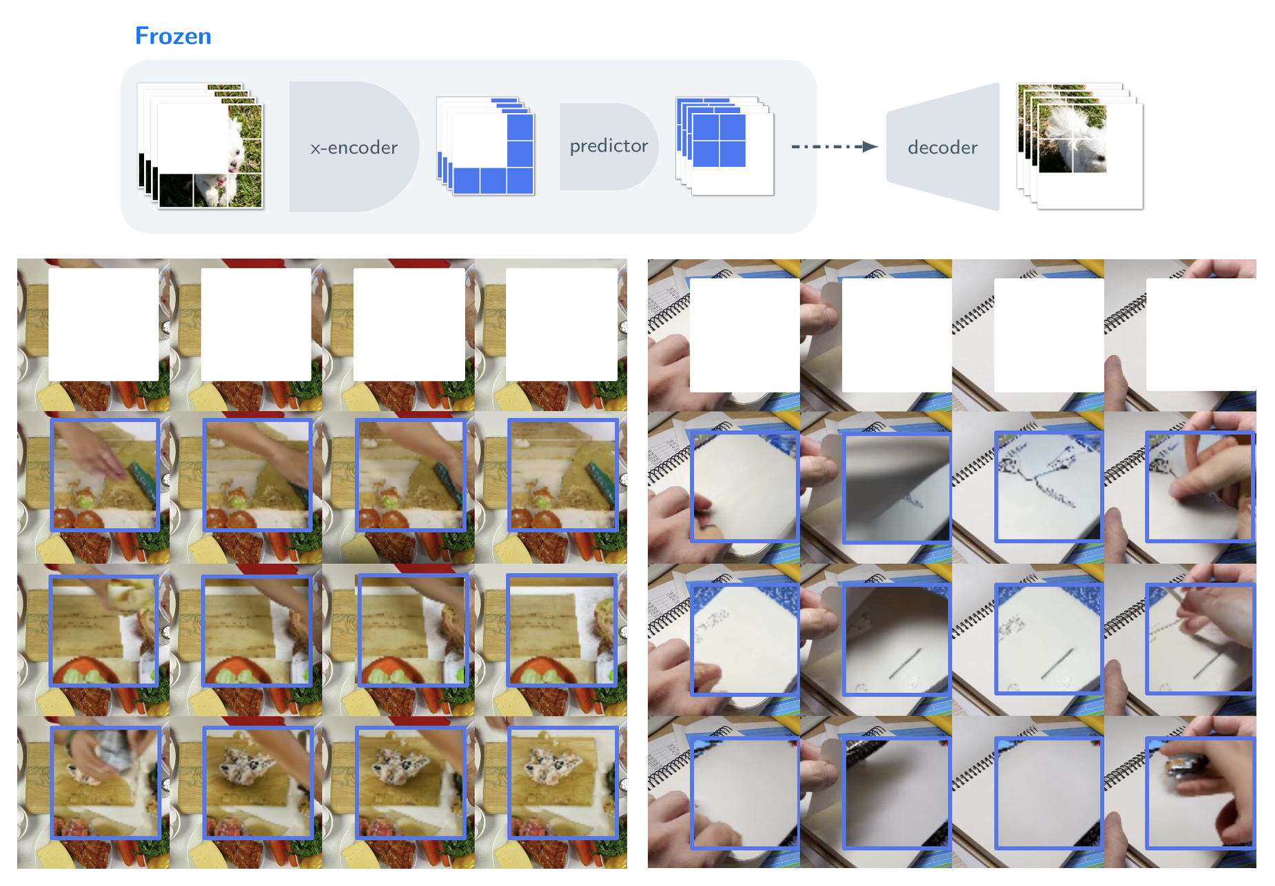
Figure 6a–6b 解读：作者冻结 V-JEPA encoder/predictor，额外训练一个 conditional diffusion model 将 predicted feature-space tokens 解码成 pixels。这个 decoder 只看到 missing regions 的 predicted features，看不到 unmasked regions，因此输出不应被理解为 V-JEPA 在做 pixel generation。多次采样中共同出现的物体轮廓、空间位置和 motion consistency，说明 V-JEPA 的 latent predictions 捕获了与可见上下文一致的语义和动态信息。

5.9 Fine-tuning 与 sample efficiency

Fine-tuning table 中：

Method	Arch.	Pretraining Data	Samples Seen	K400	SSv2
VideoMAEv1	ViT-L/16	K400/SSv2	380M/410M	85.4	74.3
VideoMAEv1	ViT-H/16	K400/SSv2	380M/410M	86.6	74.8
VideoMAEv2	ViT-H/16	Un.Hybrid	1600M	86.9	76.8
MVD	ViT-L/16	K400+IN1K	2400M	86.4	76.7
MVD	ViT-H/16	K400+IN1K	2400M	87.2	77.3
V-JEPA	ViT-L/16	VideoMix2M	270M	85.6	75.1
V-JEPA	ViT-H/16	VideoMix2M	270M	86.6	77.0

V-JEPA-H/16 在 SSv2 fine-tuning 上达到 77.0，超过 VideoMAEv2-H 的 76.8，接近 MVD-H 的 77.3；K400 上则落后 MVD-H 的 87.2。结合 sample efficiency table，V-JEPA-H/16 $_{384}$ 处理 210M samples，而 OpenCLIP / DINOv2 / VideoMAEv2 分别为 39000M / 1900M / 1600M。论文想传达的是：latent feature prediction 不是在每个任务上绝对压倒所有大模型，而是在 video motion representation 与样本效率上给出强证据。

5.10 Limitations and caveats

第一，V-JEPA 的优势主要体现在 frozen video representation，尤其是 SSv2 这类 motion-heavy task；在 image-centric tasks 上，DINOv2 / OpenCLIP 等强 image pretraining 仍明显更强。第二，论文的 qualitative decoder 是离线可视化工具，不是 V-JEPA 训练目标的一部分，因此不能把图 6 解读为“V-JEPA 是视频生成模型”。第三，released configs 使用 placeholder dataset paths；训练超参数可复现，但实际 VideoMix2M 构建仍需要研究者自己准备 HowTo100M、Kinetics、SSv2 的索引与去重。第四，frozen results 强依赖 attentive probe 和 multi-view protocol；若只用 linear probe 或单 clip，分数会显著降低。第五，论文没有给出完整 failure case taxonomy，例如极长时程、复杂因果互动、不可见物体状态等是否能被 short 16-frame clip 的 feature prediction 捕获仍不清楚。

总体结论是：V-JEPA 证明了 feature prediction 可以作为 video self-supervised learning 的独立目标，在不依赖 text、negative samples、pretrained teacher 或 pixel reconstruction 的情况下，学出对 appearance 与 motion 都有用的 visual representations。它把 JEPA/world-model 思路落到了一个现代 ViT video pretraining setting 中，并用 code release 中的 multi-block masks、EMA target encoder、narrow predictor 和 attentive probing 形成了一套可复现实验基线。

Paper Notes

探索

Revisiting Feature Prediction for Learning Visual Representations from Video

Revisiting Feature Prediction for Learning Visual Representations from Video

1. Motivation (研究动机)

2. Idea (核心思想)

3. Method (方法)

3.1 Overall framework：从 JEPA 到 V-JEPA

3.2 视频 tokenization 与 3D patch 表示

3.3 Multi-block masking：预测什么、从什么预测

3.4 V-JEPA loss 的逐步定义

3.5 Predictor 与 target encoder 的实现细节

3.6 Source-grounded pseudocode

4. Experimental Setup (实验设置)

Pretraining datasets and scale

Baselines

Metrics and protocols

Training config from released launch configs

`configs/pretrain/vitl16.yaml`

`configs/pretrain/vith16.yaml`

`configs/pretrain/vith16_384.yaml`

5. Experimental Results (实验结果)

5.1 Feature targets beat pixel targets under the same ViT-L/16 setup

5.2 Pretraining data scale: average performance improves with VideoMix2M

5.3 Pooling matters: attentive probe is not a cosmetic detail

5.4 Masking strategy ablation: multi-block 最强

5.5 与 pixel prediction methods 的同架构比较

5.6 与 state-of-the-art image/video models 的比较

5.7 Low-shot 与 temporal coverage

5.8 Qualitative visualization：V-JEPA 不是生成模型，但 predicted features 有时空一致性

5.9 Fine-tuning 与 sample efficiency

5.10 Limitations and caveats

目录