Nano World Models: A Minimalist Implementation of Future Video Prediction

Paper: arXiv:2605.23993 Code: simchowitzlabpublic/nano-world-model Code reference: main @ 63052ceb (2026-05-25)

1. Motivation (研究动机)

当前 World Model 研究的主要瓶颈

这篇 paper 的出发点不是再提出一个全新的 video diffusion trick，而是指出一个更工程化、也更科学的问题：现代 World Model 已经能在工业级系统中展示很强的 interactive video generation / future prediction 能力，但学术社区缺少一个足够小、可复现、可扩展、能系统拆解设计选择的实现。作者认为 World Model 的核心技术栈正在逐渐收敛到 video diffusion、Diffusion Forcing、consistency distillation 等相对稳定的组件；下一阶段更重要的问题不是只堆新模块，而是回答“哪些设计选择真的重要”。

具体瓶颈有三类：

实现碎片化：datasets、training recipes、evaluation protocols、downstream tasks 分散在不同 repo 或 paper 中；如果研究者想比较 prediction target、model scale、action injection、latent space，往往需要跨多个代码库重写训练 / 采样 / 评估。
实验变量纠缠：很多系统同时改变 architecture、objective、data、rollout procedure，使得结果很难归因。例如一个模型长 rollout 好，可能来自更强 backbone，也可能来自 sampling budget 或 latent representation，而不是某个单独算法。
缺少“world model as tool”的统一接口：future video prediction 本身只是第一步；同一个预测模型还应能服务 realtime simulation、MPC planning、video-to-3D reconstruction 等下游工具，但现有实现往往只覆盖单一任务。

这篇 paper 要解决的问题

作者提出 Nano World Models（NanoWM），目标是提供一个 minimalist、batteries-included 的 future video prediction / world modeling codebase。它以 Diffusion Forcing 为核心接口，把 generative objective、model scale、action-conditioning mechanism、latent observation space、dataset/environment、evaluation protocol、long-horizon rollout 都纳入同一套 Hydra 配置与训练采样管线中。

换句话说，这篇 paper 不是把 World Model 问题定义成“训练一个最强视频模型”，而是把它定义成“构造一个可控实验平台”：让研究者能在同一框架中切换 $x$ / $ϵ$ / $v$ / flow prediction、NanoWM-S/B/L/XL、additive / AdaLN / FiLM / cross-attention action injection、VAE / Web-DINO / V-JEPA latent space，并观察它们对 prediction quality、autoregressive rollout、planning success 的影响。

为什么值得研究

如果这个平台成立，它能把 World Model 从“展示 demo 的大系统”转成“可做科学实验的 substrate”。这有两层价值：

研究价值：同一套 loader / model / sampler / evaluator 让 ablation 更干净，能更可靠地判断 prediction target、latent space、action conditioning 等因素是否真的有效。
应用价值：同一模型接口可以被用作 video predictor、3D scene asset generator、MPC simulator。World Model 不只是生成未来帧，而是变成可以被下游 planner / reconstruction tool 调用的 tool。

2. Idea (核心思想)

核心洞察

NanoWM 的核心洞察是：World Model 的很多研究问题可以被统一成“对带条件的 latent video sequence 做 Diffusion Forcing”。只要把不同帧放在不同 noise level，并把 action / text / goal 等条件接入同一个 transformer backbone，同一个训练和采样接口就能覆盖 teacher-forced prediction、masked future prediction、autoregressive rollout、planning rollout 等场景。

关键创新

以 Diffusion Forcing 作为统一抽象：模型不再只一次性生成整段未来，而是允许同一 trajectory 中不同 frame 位于不同 denoising stage；context frame 可以保持 clean，future frame 可以处在更高 noise level。
把设计轴都配置化：objective、backbone scale、latent codec、action injection、dataset、evaluation、rollout length 都可以通过 config 切换，而不是在多个代码库中分别实现。
把 World Model 暴露成 tool-use interface：模型输出的 future rollout 可以继续送入 3D reconstruction，也可以在 CEM-style MPC 中作为 batched simulator 评估 action sequence。

与已有方法的根本差异

与只发布单一 task / 单一 dataset 的 video prediction repo 不同，NanoWM 的重点是“可控比较”。例如 Diffusion Forcing Transformer（DFoT）或 DINO-WM 更像特定方法或特定 latent/planning setting；NanoWM 则把这些方法背后的共性抽出来，提供统一 dataset/environment API、Diffusion Forcing sampler、action-conditioned transformer 和 evaluation scripts。它牺牲的是 SOTA 大模型规模，换来的是可复现、可替换、可诊断的实验平台。

3. Method (方法)

3.1 Overall framework：NanoWM 的总框架

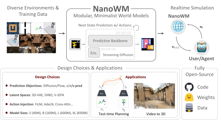
Figure 1 解读：这张 overview 图展示 NanoWM 的完整接口：左侧是多种 training data / environments，中间是 modular NanoWM，右侧是 realtime simulation、planning、video-to-3D 等用途。关键不是某个单独模块，而是所有模块都汇入同一个 Diffusion Forcing prediction interface：observation 先被编码到 latent space，模型基于 context frame 与 action condition 预测 future latent，再由 decoder 或下游 tool 使用。

整体 pipeline 可以拆成五步：

Observation encoding：输入 observation $o_{t}$ 不一定直接用 RGB，而是先编码成 $x_{t} = enc_{ψ} (o_{t})$ 。支持 Stable Diffusion VAE、Web-DINO、V-JEPA 2.1 等 latent space。
Conditional sequence modeling：给定历史 latent $x_{1 : T}$ 与条件 $c$ （例如 action sequence 或 text），学习 $p_{θ} (x_{T + 1 : T + H} ∣ x_{1 : T}, c)$ 。
Diffusion Forcing training/sampling：同一段 trajectory 中，不同 frame 可有不同 noise index $k_{t}$ ，从而统一 teacher forcing、masked future prediction 与 autoregressive rollout。
Action-conditioned transformer：NanoWM 用 latent video tokens 上的 transformer backbone；action 可以通过 additive、AdaLN、AdaLN-fuse、FiLM、cross-attention 注入。
Tool interface：生成的 future rollout 可直接作为 video prediction，也可被导出到 3D reconstruction pipeline，或作为 MPC 的 batched world simulator。

直觉上，这种设计有用是因为 future prediction 的困难不只来自生成质量，也来自实验系统的不统一。Diffusion Forcing 把“哪些 frame 是条件，哪些 frame 要生成，生成到哪个 denoising stage”显式变成 schedule；Hydra config 把“换模型 / 换 latent / 换 action injection / 换 dataset”变成小改动。于是同一个 code path 可以支持从简单 Maze 到 RT-1 robot video 的比较，降低变量混杂。

3.2 Preliminaries：world modeling 的概率形式

论文把 world modeling 定义为高维 observation sequence 的 posterior modeling。给定过去 observations $o_{1}, \dots, o_{T}$ 与条件 $c$ ，目标是补全未来 observations $o_{T + 1}, \dots, o_{T + H}$ 。实际中模型预测的是 latent： $x_{t} := enc_{ψ} (o_{t}) .$ 真实条件分布写作： $p^{⋆} (x_{T + 1 : T + H} ∣ x_{1 : T}, c),$ 学习到的模型写作： $\hat{x}_{T + 1 : T + H} \sim p_{θ} (\cdot ∣ x_{1 : T}, c) .$ 当 World Model 用于 planning 时，给定候选 action sequence $a_{T : T + H - 1}$ 与 reward / utility $R$ ，planning 目标是： $a_{T : T + H - 1}^{⋆} \in ar g max_{a_{T : T + H - 1} \in A^{H}} E_{\hat{x}_{T + 1 : T + H} \sim p_{θ} (\cdot ∣ x_{1 : T}, c, a_{T : T + H - 1})} [R (\hat{x}_{T + 1 : T + H}, a_{T : T + H - 1})] .$ 这一定义把 World Model 明确接到 MPC：模型只负责预测 rollout，planner 负责搜索 action，reward/objective 可以因任务而变。

3.3 Diffusion Forcing：统一 training 与 rollout 的接口

Diffusion Forcing 的关键设定是给每一帧一个 noise index。设 noise index set 为 $K \subset R$ ，对 encoded trajectory $x_{1 : T + H}$ ，每一帧 $x_{t}$ 都有对应 $k_{t} \in K$ ，schedule 为： $k = (k_{1}, \dots, k_{T + H}) .$ 训练时模型看到 noised trajectory 与 noise-index schedule。context frames 可以保持 clean 或 nearly clean，future frames 可以被赋予更高 noise。只改变 schedule，就可以表达不同模式：

Teacher-forced prediction：context 与一部分 future 保持低噪声，模型学习局部预测。
Masked future prediction：未来帧高噪声，模型从 context 中补全。
Autoregressive rollout：每次生成一小段，再把生成结果滑入下一次 context window。

这就是 NanoWM 能把训练、验证、long rollout、planning rollout 复用同一 sampler 的原因。

3.4 Generative objectives： $x$ / $ϵ$ / $v$ / flow prediction

NanoWM 在同一 Diffusion Forcing interface 下支持多种 generative objective：

$x$ -prediction：模型直接预测 clean latent $x_{0}$ / $x_{start}$ 。
$ϵ$ -prediction：模型预测加到 latent 上的 Gaussian noise。
$v$ -prediction：模型预测 velocity-style target；released code 中 GaussianDiffusion.training_losses 通过 _predict_v(x_start, t, noise) 构造 target。
Flow matching：模型预测 data-noise interpolant 诱导的 velocity field；released code 中 src/diffusion/flow_matching.py 提供对应实现，dino_wm_pusht_flow.yaml 把 pred_name 设为 flow。

这些 objective 的共同点是 backbone、dataset loader、conditioning interface、sampling code 不变，只改变 noised input 与 target construction。released code 中 src/diffusion/gaussian_diffusion.py::training_losses 的核心逻辑是：先用 q_sample 得到 $x_{t}$ ，再根据 PredName 选择 target：START_X -> x_start、EPSILON -> noise、V -> _predict_v(...)，最后对 model output 与 target 做 MSE，并可加 Min-SNR weighting。

3.5 NanoWM architecture：latent video transformer + action injection

NanoWM 使用 transformer backbone 处理 latent video tokens。对 VAE-style encoding，每帧 latent 会被分成 spatial patches，投影到 hidden dimension，再经过 interleaved spatial-temporal attention。命名规则类似 image/video diffusion model：NanoWM-B/2 表示 Base family、latent patch size 为 2；NanoWM-B/4、NanoWM-B/8 使用更粗的 latent patch。

released code 中模型 family 的实际定义在 src/models/nanowm.py：

NanoWM-S/*：depth 12，hidden size 384，heads 6。
NanoWM-B/*：depth 12，hidden size 768，heads 12。
NanoWM-L/*：depth 24，hidden size 1024，heads 16。
NanoWM-XL/*：depth 28，hidden size 1152，heads 16。

Action conditioning 对 world model 很关键，因为模型需要回答“如果执行这串 actions，未来会怎样”。NanoWM 支持五种 action injection：

additive：把 action embedding 加到对应 frame tokens 上；参数最少，是默认强 baseline。
AdaLN：用 action 调制 layer norm 参数。
AdaLN-fuse：把 action 与 timestep conditioning 融合。
FiLM：用 action 产生 feature-wise modulation。
cross-attention：video tokens 通过 cross-attention 读取 action tokens。

代码中 TransformerBlock 显式支持 additive、adaln_fuse、adaln、film、cross_attention。在 NanoWM.forward 中，action 先过 ActionEmbedder，再根据 injection type 走不同分支：adaln_fuse 会把 action embedding 加进 timestep embedding c，其他类型则把 action_emb 传入 spatial / temporal transformer block。

3.6 Latent observation spaces：VAE vs semantic features

NanoWM 支持三类 latent observation space：

SD-VAE：重建导向，可以 decode 回 RGB，因此适合 video generation、PSNR/SSIM/LPIPS/FID 评估，也更适合目标状态要在视觉空间对齐的 planning。
Web-DINO：自监督 semantic/geometric representation，理论上对 downstream prediction 和 planning 有吸引力。
V-JEPA 2.1：video-pretrained predictive visual features，更偏 representation learning。

论文的实验表明，semantic latent 不会自动带来更好的 planning：在 PushT planning 中，SD-VAE latent 有 25.0% success rate，而 Web-DINO 与 V-JEPA 2.1 都是 0.0%。作者进一步用 ground-truth action rollout diagnostic 说明 semantic-latent checkpoint 几乎没有学会使用 action input。

3.7 Dataset / environment interface

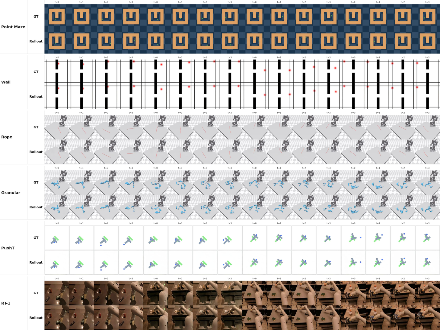
Figure 2 解读：这张图把 GT sequence 与 NanoWM rollout 放在一起，覆盖 Point Maze、Wall、Rope、Granular、PushT、RT-1。它说明 NanoWM 的 dataset/environment interface 并不只服务一个 domain：grid-world navigation、deformable manipulation、tabletop pushing、real-robot video 都被统一成可训练 / 可采样的 trajectory 数据。图中不同 domain 的视觉复杂度逐渐上升，也对应后续结果中 PSNR/SSIM/LPIPS/FID 的明显差异。

支持的 environment / dataset 包括：

DINO-WM style environments：Point Maze、Wall、PushT、Rope、Granular。代码配置在 src/configs/dataset/dino_wm/*.yaml，例如 PushT 使用 frame_interval=5、2D action、relative action、action_scale=100.0。
CS:GO game simulation：配置 src/configs/experiment/csgo.yaml 使用 50K steps、batch size 6、learning rate 1e-5；CSGO-specific model 使用 16-frame window、4 context frames。
RT-1 / Fractal robot data：src/configs/dataset/rt1/rt1.yaml 指向 IPEC-COMMUNITY/fractal20220817_data_lerobot，action dim 为 7；代码注释说明训练集约 87K episodes，并使用 random slice sampling。

3.8 Evaluation / logging / reproducibility

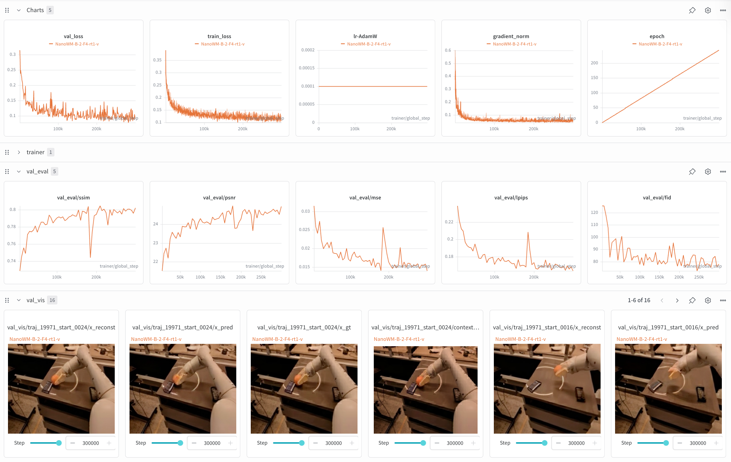
Figure 3 解读：这张图展示 Weights & Biases 中的训练曲线、validation metrics 和 qualitative prediction panels。NanoWM 的重点是把 logging / checkpoint / evaluation 都纳入同一 callback-style pipeline：同一 run 里同时记录 PSNR、SSIM、LPIPS、FID、reconstruction videos、predicted rollouts、ground-truth clips。这对“可科学比较”很重要，因为 ablation 需要固定 seed、固定 validation clips、固定 evaluation code，而不是只看 cherry-picked rollout。

标准 evaluation protocol：除非特别说明，使用 256 fixed validation clips、seed 42、autoregressive sequential scheduling。标准 256-resolution model 每个 validation clip 有 4 frames：1 个 context frame + 3 个 generated frames；metrics 只在 generated frames 上计算。diffusion models 默认使用 250 DDIM sampling steps。

3.9 Long-horizon rollout

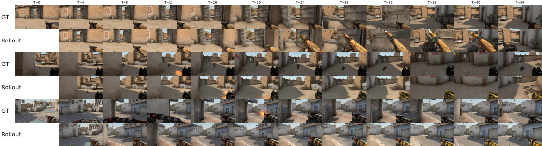
Figure 5 解读：这张图展示 CSGO checkpoint 的 50-frame autoregressive long rollout。模型从 4 个 ground-truth history frames 初始化，然后逐帧生成剩余 46 帧。可见 coarse scene geometry 与 camera motion 能保持一段时间，但 weapon appearance、local texture 等细节会逐渐漂移，说明 autoregressive rollout 的主要问题是误差累积而不是第一步预测完全失败。

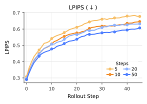
Figure 6 解读：LPIPS 曲线把 Figure 5 的现象量化：随着自生成 rollout 变长，perceptual error 逐步上升；增加 DDIM sampling steps 可以降低整个 rollout horizon 上的 LPIPS。这支持 Finding #5：更强的 per-frame denoising 能部分缓解 autoregressive compounding error，但不能从根本上消除误差累积。

released code 的 long rollout launch script src/scripts/eval/long_rollout_csgo.sh 与论文描述一致：默认 ROLLOUT_LENGTH=50、HISTORY_LENGTH=4、NUM_SAMPLING_STEPS=50、SCHEDULING_MODE=sequential，checkpoint 路径指向 CSGO 100K latest ckpt。src/sample/rollout.py 实现 sliding window：每一步取最近 history_length 个 latent 与对应 action window，调用 dfot_sample(..., n_generate_frames=1)，再把新 latent 拼回 generated sequence。

3.10 World-modeling as tool-use：3D export 与 MPC

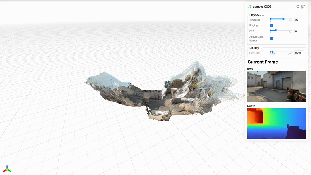
Figure 4 解读：这张图说明 NanoWM 的 rollout 可以被当成下游 3D pipeline 的输入：CSGO 生成帧先 decode 成 RGB，再交给 depth / camera estimation pipeline，输出 estimated depth 与 persistent point cloud。这里 NanoWM 不绑定某个 3D backend；它只负责生成时间一致的 visual rollout，几何估计由外部工具完成。

MPC planning 中，NanoWM 被包装为 batched rollout function。planner 接收当前 observation context、goal specification 和一组 candidate action sequences；world model 并行预测每个 action sequence 的 future trajectory；objective module 根据 goal distance、task progress 或 task-specific reward 给出 scalar score；CEM 更新 action distribution，执行最优 sequence 的第一个 action，然后重新观测与 replanning。

论文公式与 released code 实现差异：论文在 latent planning 文字中写到使用 64 CEM samples 和 5 CEM iterations；但 released code 的 src/scripts/eval/planning_pusht.sh 调用 planning=dino_wm_pusht，对应 src/configs/planning/dino_wm_pusht.yaml 里是 num_samples=300、topk=30、opt_steps=30、num_sampling_steps=20。src/configs/planning/base.yaml 也写的是 num_samples=100、topk=10、opt_steps=30。我未在 released code path 中找到与 paper 64/5 完全一致的 shipped config；因此 note 中把 paper 表格设置与 released config 分开记录。

3.11 Pseudocode：基于 released code 的关键组件

下面 pseudocode 不是复述 abstract，而是按 main@63052ceb 的实际代码路径抽象。

A. Diffusion Forcing training step

import torch
import torch.nn.functional as F
 
 
def nanowm_training_step(model, diffusion, batch, timestep_sampler, pred_name="v"):
    # src/experiments/train_experiment.py::NanoWMTrainingModule.training_step
    # batch contains latent/video tensor x and optional action tensor
    x = batch["video_latents"]              # [B, F, C, H, W]
    action = batch.get("action", None)      # [B, F, action_dim] or None
 
    # sample one timestep/noise index per frame for Diffusion Forcing
    t = timestep_sampler.sample(batch_size=x.shape[0], num_frames=x.shape[1])
    model_kwargs = {"action": action} if action is not None else {}
 
    # src/diffusion/gaussian_diffusion.py::training_losses
    noise = torch.randn_like(x)
    x_t = diffusion.q_sample(x_start=x, t=t, noise=noise)
    model_output = model(x_t, t, **model_kwargs)
 
    if pred_name == "x":
        target = x
    elif pred_name == "eps":
        target = noise
    elif pred_name == "v":
        target = diffusion._predict_v(x_start=x, t=t, noise=noise)
    else:
        raise ValueError(pred_name)
 
    loss = F.mse_loss(model_output, target, reduction="none")
    return loss.flatten(1).mean(1).mean()

B. Action-conditioned NanoWM forward

import torch
from einops import rearrange
 
 
def nanowm_forward(x, timesteps, spatial_blocks, temporal_blocks, action=None,
                   action_injection_type="additive"):
    # src/models/nanowm.py::NanoWM.forward / TransformerBlock
    # x: [B, F, C, H, W]
    B, F, C, H, W = x.shape
    tokens = patch_embed(x)                         # [B*F, N, D]
    c = timestep_embed(timesteps).reshape(B * F, -1)
 
    action_emb = None
    if action is not None:
        action_emb = action_embedder(action)         # [B, F, D]
        action_emb = action_emb.reshape(B * F, 1, -1)
 
    for spatial_block, temporal_block in zip(spatial_blocks, temporal_blocks):
        spatial_action = None
        temporal_action = None
 
        if action_emb is not None:
            if action_injection_type == "adaln_fuse":
                c = c + action_emb.squeeze(1)        # fuse action into timestep condition
            else:
                spatial_action = action_emb          # additive / adaln / film / cross_attention
 
        tokens = spatial_block(tokens, c, action_emb=spatial_action, is_causal=False)
        tokens = rearrange(tokens, "(b f) n d -> (b n) f d", b=B)
        tokens = temporal_block(tokens, c, action_emb=temporal_action, is_causal=True)
        tokens = rearrange(tokens, "(b n) f d -> (b f) n d", b=B)
 
    return final_layer(tokens, c)

C. DFOT sequential sampling / long rollout

import torch
 
 
def long_rollout(diffusion, model, init_context, actions, rollout_length=50,
                 history_length=4, num_sampling_steps=50):
    # src/sample/rollout.py + src/diffusion/df_sample.py
    generated = init_context.clone()  # first 4 frames are ground-truth history
 
    for t in range(history_length, rollout_length):
        context = generated[:, t - history_length:t]
        action_window = actions[:, t - history_length:t]
 
        pred_latents = dfot_sample(
            diffusion=diffusion,
            model=model.forward,
            shape=(context.shape[0], history_length + 1, *context.shape[2:]),
            context=context,
            n_context_frames=history_length,
            model_kwargs={"action": action_window},
            scheduling_mode="sequential",
            num_sampling_steps=num_sampling_steps,
            n_generate_frames=1,
            history_stabilization_level=0.02,
        )
        new_latent = pred_latents[:, history_length:history_length + 1]
        generated = torch.cat([generated, new_latent], dim=1)
 
    return generated[:, :rollout_length]

D. CEM-style MPC planning with world model rollout

import torch
 
 
def cem_plan(world_model, objective_fn, obs_0, goal, action_dim, horizon,
             num_samples=300, topk=30, opt_steps=30, sigma_min=1e-3):
    # src/planning/cem_planner.py and src/planning/diffusion_world_model.py
    mu = torch.zeros(horizon, action_dim)
    sigma = torch.ones(horizon, action_dim)
    z_goal = world_model.encode_obs(goal)
 
    for _ in range(opt_steps):
        action_samples = mu + sigma * torch.randn(num_samples, horizon, action_dim)
        pred_rollouts = world_model.rollout(
            obs_0=obs_0,
            act=action_samples,
            num_sampling_steps=20,
        )
        loss = objective_fn(pred_rollouts, z_goal)   # lower is better
        topk_idx = torch.argsort(loss)[:topk]
        elite = action_samples[topk_idx]
        mu = elite.mean(dim=0)
        sigma = elite.std(dim=0).clamp(min=sigma_min)
 
    return mu[0]  # execute first action, then observe and replan

3.12 Code-to-paper mapping

Code reference: main @ 63052ceb (2026-05-25) — pseudocode and mapping based on this commit

Paper Concept	Source File	Key Class/Function
Hydra entrypoint / task dispatch	`src/main.py`	`main(cfg)`
Training loop and validation callback	`src/experiments/train_experiment.py`	`NanoWMTrainingModule.training_step`, `validation_step`
Diffusion objectives: $x$ / $ϵ$ / $v$	`src/diffusion/gaussian_diffusion.py`	`GaussianDiffusion.training_losses`, `PredName`
Flow matching objective	`src/diffusion/flow_matching.py`; `src/configs/experiment/dino_wm_pusht_flow.yaml`	`FlowMatching`, `pred_name: flow`
Diffusion Forcing schedule / sampler	`src/diffusion/df_sample.py`	`generate_sequential_schedule`, `generate_full_sequence_schedule`, `dfot_sample`
NanoWM transformer backbone	`src/models/nanowm.py`	`NanoWM`, `TransformerBlock`, `NanoWM_B_2`, `NanoWM_L_2`
Action injection variants	`src/models/nanowm.py`; `src/configs/model/nanowm_b2.yaml`	`ActionEmbedder`, `action_injection.type`
Dataset/environment configs	`src/configs/dataset/dino_wm/*.yaml`, `src/configs/dataset/rt1/rt1.yaml`	frame intervals, action dims, loader paths
Standard metrics evaluation	`src/sample/evaluate_metrics.py`; `src/utils/metrics.py`	PSNR, SSIM, LPIPS, FID/FVD utilities
Long-horizon rollout	`src/sample/rollout.py`; `src/scripts/eval/long_rollout_csgo.sh`	sliding history window + `dfot_sample`
MPC planning wrapper	`src/planning/diffusion_world_model.py`	`DiffusionWorldModel.rollout`
CEM planner and objective	`src/planning/cem_planner.py`, `src/planning/objective.py`	top-k CEM update, goal latent objective

4. Experimental Setup (实验设置)

Datasets and scale

DINO-WM environments：Point Maze、Wall、Rope、Granular、PushT。论文未详细说明每个 environment 的 raw sample count；released configs 给出 frame/action settings，例如 PushT 使用 frame_interval=5、2D relative actions、action_scale=100.0。
RT-1 / Fractal：论文在 ablation 中使用 RT-1 fractal；released src/configs/dataset/rt1/rt1.yaml 指向 IPEC-COMMUNITY/fractal20220817_data_lerobot，action dim 为 7，代码注释写训练集约 87K episodes。
CS:GO：用于 game simulation 和 long-horizon rollout；论文未详细说明 raw dataset count。CSGO-specific config 使用 16-frame training windows 与 4 context frames。
Evaluation clips：标准 evaluation 使用 256 fixed validation clips，seed 42；标准 256-resolution models 条件为 1 context frame + 3 generated frames。

Compared baselines / variants

这篇 paper 主要做内部 controlled ablation，而不是与一组外部 SOTA baseline 做排行榜比较。比较对象包括：

Prediction target： $v$ -prediction、 $x$ -prediction、 $ϵ$ -prediction。
Model scale：NanoWM-S/2、NanoWM-B/2、NanoWM-L/2。
Action injection：additive、AdaLN、AdaLN-fuse、FiLM、cross-attention。
Latent space：SD-VAE、Web-DINO、V-JEPA 2.1。
Sampling budget / long rollout：不同 DDIM steps 下的 LPIPS accumulation。

Evaluation metrics

PSNR：pixel-level reconstruction fidelity，越高越好。
SSIM：结构相似度，越高越好。
LPIPS：perceptual distance，越低越好。
FID：generated frames 与 ground-truth validation frames 的分布距离，越低越好。
FVD：用于足够长的视频，衡量 temporal video distribution similarity；论文只在 setup 中说明。
Planning success rate：PushT 中 final state 是否满足 environment-specific goal condition。
Latent MSE / cosine distance：用于诊断 final predicted latent 与 goal latent 的距离，判断模型是否真的使用 action input。

Training config / hardware / hyperparameters

RT-1 target / scale / action-injection ablations：论文写明使用 NanoWM-B/2、SD-VAE、element-wise addition 默认 action injection；每个 run 训练 50K steps，8 GPUs，每 GPU batch size 8，有效 batch size 64，1 context frame + 3 future frames。released code 对应 src/configs/experiment/ablation_rt1.yaml：max_steps=50000、batch_size=8、num_workers=16；src/configs/model/nanowm_b2.yaml：num_frames=4、n_context_frames=1、num_sampling_steps=250、latent_size=32、latent_channels=4。
Standard model defaults：src/configs/experiment/default.yaml 使用 Adam-style optimizer LR 1e-4、weight decay 0.01、warmup 1000、gradient clip norm 0.1、default diffusion steps 1000、default pred_name=v、snr_gamma=5.0、zero_terminal_snr=true、history_stabilization_level=0.02。
DINO-WM shipped checkpoints：Point Maze 30K、Wall 15K、Rope 15K、Granular 15K、PushT 100K；对应 config files src/configs/experiment/dino_wm_*.yaml。
RT-1 shipped checkpoint：src/configs/experiment/rt1.yaml 使用 max_steps=300000、batch size 8、8 GPUs（论文说明）。
CSGO：src/configs/experiment/csgo.yaml 使用 max_steps=50000、batch size 6、LR 1e-5；long rollout script 默认 checkpoint 为 CSGO 100K latest ckpt，rollout length 50、history length 4、DDIM steps 50。
Planning：paper latent planning 表格写 goal horizon $H = 3$ 、64 CEM samples、5 CEM iterations；released dino_wm_pusht.yaml planning config 使用 horizon 5、replan every 5、50 evals、300 samples、top-30、30 iterations、20 DDIM steps。

5. Experimental Results (实验结果)

5.1 Prediction target ablation on RT-1 fractal

Target	Schedule	PSNR ↑	SSIM ↑	LPIPS ↓	FID ↓
$v$	cosine + ZTSNR	23.07	0.760	0.207	42.27
$x$	cosine + ZTSNR	23.37	0.783	0.184	42.99
$ϵ$	linear	21.89	0.739	0.225	48.86

Finding #1： $ϵ$ -prediction 在这组 schedule 下明显落后； $x$ -prediction 的 reconstruction metrics 最好， $v$ -prediction 的 FID 更好且是 NanoWM 默认设置。作者特别说明， $x$ 和 $v$ 使用 squared-cosine + ZTSNR，而 $ϵ$ 使用 linear schedule，因为 cosine + ZTSNR 在 terminal timestep 上对 $ϵ$ -prediction 数值不稳定。

5.2 Model scale ablation on RT-1 fractal

Architecture	Params	PSNR ↑	SSIM ↑	LPIPS ↓	FID ↓
NanoWM-S/2	39.8M	22.30	0.739	0.230	54.95
NanoWM-B/2	158.6M	23.07	0.760	0.207	42.27
NanoWM-L/2	~460M	23.62	0.777	0.186	36.31

Finding #2：model scale 带来单调收益，从 S/2 到 B/2 到 L/2，PSNR、SSIM、LPIPS、FID 全部改善。这说明在统一训练 recipe 下，capacity 仍然是 future video prediction 的重要因素。

5.3 Action-injection ablations

RT-1：

Method	PSNR	SSIM	LPIPS	FID	Params
additive	23.07	0.760	0.207	42.27	158.6M
AdaLN	23.19	0.762	0.206	43.62	158.6M
AdaLN-fuse	23.10	0.762	0.206	43.03	158.6M
FiLM	23.20	0.763	0.203	40.62	172.8M
cross-attention	20.82	0.721	0.242	51.12	187.0M

PushT：

Method	PSNR	SSIM	LPIPS	FID	Extra params
additive	26.20	0.962	0.053	23.89	0
AdaLN-fuse	26.17	0.961	0.051	30.28	0
AdaLN	26.09	0.960	0.053	26.32	~42.5M
cross-attention	25.95	0.959	0.055	28.64	~28.3M
FiLM	25.88	0.960	0.056	25.45	~14.4M

Finding #3：action injection 是 task-dependent。FiLM 在 RT-1 上视觉指标最好，但简单 additive 在 PushT 上整体最强且没有额外参数；cross-attention 在 RT-1 上反而明显退化。这个结果提醒：更复杂的 conditioning 不一定更好，尤其当 action 与视觉 dynamics 的耦合方式较简单时，轻量 additive 可能更稳。

5.4 Latent space and planning

Goal-conditioned planning on PushT：

Latent space	Backbone	Latent shape	Success rate
SD-VAE	NanoWM-B/2	[4, 32, 32]	25.0%
Web-DINO	NanoWM-B/1	[1024, 16, 16]	0.0%
V-JEPA 2.1	NanoWM-B/1	[1024, 16, 16]	0.0%

Ground-truth action rollout diagnostic on PushT（32 goal-reaching episodes， $H = 3$ ，20 DDIM steps）：

Latent space	MSE init ↓	MSE GT action ↓	MSE zero action ↓	MSE random action ↓	Cos init ↓	Cos GT action ↓	Cos zero action ↓	Cos random action ↓
SD-VAE	0.077714	0.014015	0.074830	0.081412	0.038073	0.008885	0.037322	0.042239
Web-DINO	0.311649	0.834037	0.834044	0.834066	0.111740	0.280007	0.280011	0.280025
V-JEPA 2.1	0.206433	0.584029	0.584056	0.584150	0.047607	0.138866	0.138872	0.138893

Action embedding magnitude：

Latent space	Action embedding RMS
SD-VAE	0.1119
Web-DINO	0.00214
V-JEPA 2.1	0.00129

Finding #4：semantic latent space 不会自动提升 planning。SD-VAE checkpoint 明显受 ground-truth actions 影响，GT action rollout 到 goal latent 的距离远小于 zero/random action；Web-DINO 与 V-JEPA 的 GT/zero/random 几乎一样，action embedding RMS 也接近 0，说明模型没有学到 counterfactual action-conditioned dynamics。

5.5 Long-horizon rollout and sampling budget

Finding #5：NanoWM 可以生成 plausibly coherent 的 long-horizon rollout，但 autoregressive generation 会随时间积累 perceptual error。CSGO long rollout 使用 4 history frames，逐帧生成 46 个未来 frames；50 DDIM steps 是 long rollout script 的默认设置。Figure 6 中 LPIPS 随 rollout horizon 增加而上升；增加 DDIM sampling budget 会降低 LPIPS，说明 per-frame denoising 更充分可以缓解但不能完全解决 compounding error。

5.6 Shipped checkpoints across domains

Dataset	Steps	PSNR ↑	SSIM ↑	LPIPS ↓	FID ↓
Point Maze	30K	36.74	0.984	0.019	9.66
Wall	15K	34.05	0.994	0.010	2.64
Rope	15K	31.63	0.953	0.056	35.20
Granular	15K	26.08	0.917	0.073	40.05
PushT	100K	33.19	0.982	0.016	13.63
RT-1	300K	24.36	0.787	0.180	35.08

Finding #6：同一 training / evaluation recipe 可以跨 navigation、tabletop pushing、deformable manipulation、real-robot video 工作，但 domain complexity 对指标影响很大。Wall / Point Maze 这类简单环境指标最好；RT-1 和 Granular 更复杂，FID/LPIPS 明显更差。这与 Figure 2 的视觉复杂度一致。

5.7 Limitations and conclusions

论文没有把 NanoWM 包装成 SOTA closed-world simulator；它的主要限制也来自 minimalist research substrate 的定位：

长程 rollout 仍有误差累积：即使 coarse geometry 和 camera motion 能维持，local texture / object details 仍会随 autoregression 漂移。
semantic latent planning 失败：Web-DINO / V-JEPA 并未自然学会 action-conditioned counterfactual prediction；如果 objective 不迫使模型使用 action，semantic representation 反而可能对 planning 不友好。
dataset scale 信息不完整：paper 对部分 raw dataset sizes 没有详细说明，复现实验需要依赖 released docs/configs/checkpoints。
released config 与 paper 部分 planning 描述不完全一致：planning CEM sample/iteration budget 需要按具体 commit 下的 configs 再确认。

总体结论是：NanoWM 的贡献不在于单项指标压倒所有方法，而在于提供了一个小而完整的 World Model science platform。它用统一 Diffusion Forcing interface 把 objective、scale、action injection、latent space、dataset、rollout、planning、3D export 连接起来，并通过 ablations 证明这些设计轴会显著影响 future video prediction 与 downstream tool-use 行为。

Paper Notes

探索

Nano World Models: A Minimalist Implementation of Future Video Prediction

Nano World Models: A Minimalist Implementation of Future Video Prediction

1. Motivation (研究动机)

当前 World Model 研究的主要瓶颈

这篇 paper 要解决的问题

为什么值得研究

2. Idea (核心思想)

核心洞察

关键创新

与已有方法的根本差异

3. Method (方法)

3.1 Overall framework：NanoWM 的总框架

3.2 Preliminaries：world modeling 的概率形式

3.3 Diffusion Forcing：统一 training 与 rollout 的接口

3.4 Generative objectives：x / ϵ / v / flow prediction

3.5 NanoWM architecture：latent video transformer + action injection

3.6 Latent observation spaces：VAE vs semantic features

3.7 Dataset / environment interface

3.8 Evaluation / logging / reproducibility

3.9 Long-horizon rollout

3.10 World-modeling as tool-use：3D export 与 MPC

3.11 Pseudocode：基于 released code 的关键组件

A. Diffusion Forcing training step

B. Action-conditioned NanoWM forward

C. DFOT sequential sampling / long rollout

D. CEM-style MPC planning with world model rollout

3.12 Code-to-paper mapping

4. Experimental Setup (实验设置)

Datasets and scale

Compared baselines / variants

Evaluation metrics

Training config / hardware / hyperparameters

5. Experimental Results (实验结果)

5.1 Prediction target ablation on RT-1 fractal

5.2 Model scale ablation on RT-1 fractal

5.3 Action-injection ablations

5.4 Latent space and planning

5.5 Long-horizon rollout and sampling budget

5.6 Shipped checkpoints across domains

5.7 Limitations and conclusions

目录

3.4 Generative objectives： $x$ / $ϵ$ / $v$ / flow prediction