LeWorldModel: Stable End-to-End Joint-Embedding Predictive Architecture from Pixels

Paper: arXiv:2603.19312 Code: lucas-maes/le-wm Code reference: main @ c8a44170 (2026-05-17)

1. Motivation (研究动机)

这篇论文要解决的是一个很具体的矛盾：JEPA / latent world model 的目标本来是“不要重建像素，只预测更抽象、更可控的未来表示”，但一旦从 raw pixels 到 encoder、predictor 全部端到端训练，最简单的 next-embedding prediction loss 会自然产生 representation collapse，encoder 可以把所有画面映射到近似常数，predictor 也就能轻松预测，却学不到任何可用于 planning 的物理状态。作者把这个问题放在 world model 的控制场景里看：如果 latent 表示既不能避免 collapse，又不能保留动作相关的状态变量，那么后续 Model Predictive Control 只是在一个错误的“想象空间”里优化动作序列。

现有路线各有代价。PLDM 代表 end-to-end pixel JEPA / latent dynamics 路线，它直接从像素联合训练 encoder 和 predictor，不依赖 frozen foundation encoder，也不需要 reward；但它为了稳定训练引入了来自 VICReg 的多项约束和额外 loss 权重，论文指出可调 loss coefficient 多达六个，调参复杂度接近 $\mathcal{O}(n^6)$，而且缺少明确的 anti-collapse 保证。DINO-WM 则用 frozen DINOv2 encoder 规避 collapse，但这样把表征学习外包给大规模预训练，牺牲了从目标环境像素端到端学习的能力，也带来大量 token 和推理成本。Dreamer、TD-MPC 等 task-specific world model 又通常需要 reward、privileged state 或任务相关监督，不符合“先从离线无奖励轨迹学习通用 dynamics，再做控制”的目标。

LeWorldModel (LeWM) 的研究价值在于，它试图把 JEPA 的几个理想属性同时放在一个小模型里：从 raw pixels 端到端训练；不重建像素、不用 reward、不用 stop-gradient、EMA teacher 或 frozen encoder；训练目标只有 next-embedding prediction 与 Gaussian latent regularization 两项；最后还要能在 2D / 3D 控制任务上直接用 latent planning。若这个目标成立，它不仅是一个更稳定的 JEPA 训练 recipe，也说明“紧凑 latent space + action-conditioned predictor”可以替代昂贵的 foundation visual tokens 来做 goal-conditioned planning。

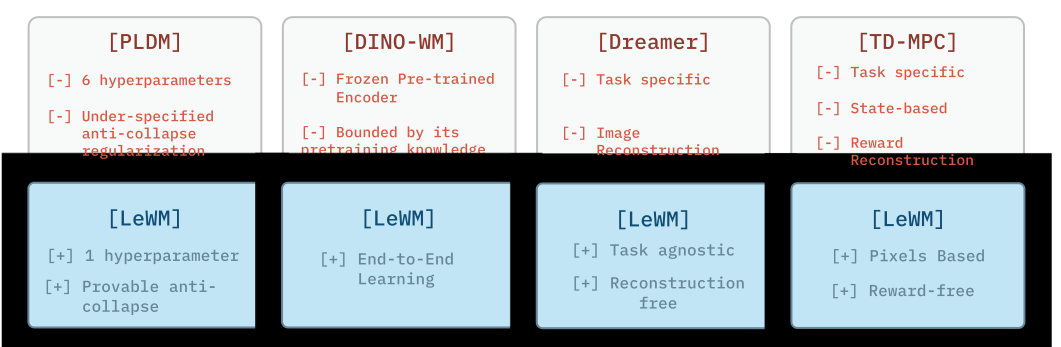
Figure 1 解读：这张图把 latent world model 分成 task-specific、foundation-based 和 end-to-end 三类。LeWM 的位置很明确：它希望保留 PLDM 的端到端与 task-agnostic 优点，但把多项正则和复杂调参替换成单个 SIGReg 系数；同时避免 DINO-WM 对 frozen DINOv2 表示的依赖。论文真正关心的不是又提出一个控制 benchmark，而是证明端到端 JEPA 可以在像素输入下稳定训练并用于 planning。

2. Idea (核心思想)

核心 insight 是：JEPA 的 collapse 不一定要靠 teacher-student、stop-gradient、reconstruction 或 foundation encoder 来解决；如果把每个时间步的 latent embedding 分布直接约束到 isotropic Gaussian，encoder 就不能把所有样本压成一个常数点，同时 prediction loss 仍然会迫使这个 Gaussian latent space 按动作组织出可预测的动力学结构。

LeWM 因此只保留两类压力：${\mathcal{L}}_{\mathrm{pred}}$ 让当前 latent 和 action 能预测下一步 latent，SIGReg 让每个 batch / time step 的 latent 分布近似 $N(0,I)$。与 PLDM 相比，LeWM 不是堆叠 variance、covariance、temporal smoothness、inverse dynamics、reconstruction 等多项启发式约束，而是用一个分布匹配统计量提供 anti-collapse；与 DINO-WM 相比，它不借助大规模预训练视觉表征，而是让 encoder 在目标环境轨迹上从零学习。

这个设计的关键差异在于“正则化对象”不是像素重建质量，也不是 reward 预测，而是 latent distribution 本身。直觉上，prediction loss 负责把 latent space 拉成“动作可预测”的形状，SIGReg 负责防止这个空间退化成低维常数或少量簇；二者共同形成一种 tension：表示既要足够分散，又要保留可预测的时序结构。

3. Method (方法)

3.1 Overall framework: 从离线轨迹学习 latent dynamics

LeWM 的输入是离线收集的轨迹：raw pixel observations ${\mathbf{o}}_{1:T}$ 和 actions ${\mathbf{a}}_{1:T}$。训练阶段没有 reward、没有 task specification，也不需要 privileged state。encoder ${\mathrm{enc}}_{\theta }$ 把每一帧映射为低维 latent ${\mathbf{z}}_t$，predictor ${\mathrm{pred}}_{\varphi }$ 在 latent space 中根据当前表示与 action 预测下一步表示： $\begin{array}{rl}\text{Encoder:}& {\mathbf{z}}_t={\mathrm{enc}}_{\theta }({\mathbf{o}}_t),\\ \text{Predictor:}& {\hat{\mathbf{z}}}_{t+1}={\mathrm{pred}}_{\varphi }({\mathbf{z}}_t,{\mathbf{a}}_t).\end{array}$

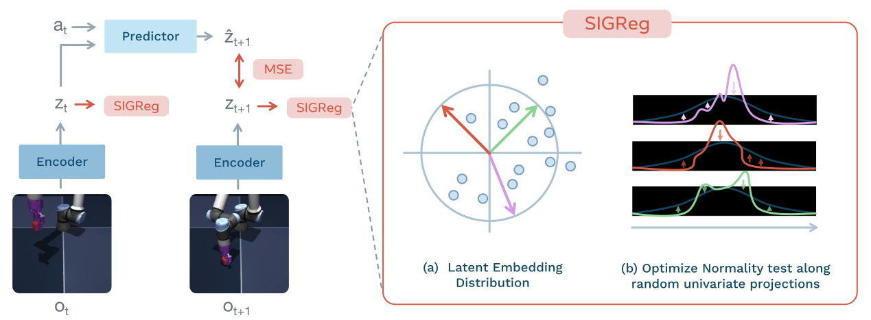
Figure 2 解读：训练 pipeline 左侧是 frame encoder，右侧是 action-conditioned predictor。每个观测帧先变成 compact latent token，predictor 在 history 上做 causal autoregressive next-latent prediction。下方的损失结构体现论文的最小化设计：预测误差让 latent 对未来有用，SIGReg 把 latent 分布推向 isotropic Gaussian 来防止 collapse。注意 decoder 不在训练目标里，后续可视化 decoder 只是诊断 latent 中保留了哪些场景信息。

方法的 intuition 可以这样理解：如果只优化 $\Vert {\hat{\mathbf{z}}}_{t+1}-{\mathbf{z}}_{t+1}{\Vert }^2$，最稳定的局部解就是所有 $\mathbf{z}$ 都一样；如果只做 Gaussian regularization，latent 会分散但未必与动作动力学对齐。LeWM 把这两个目标叠加后，encoder 必须在 Gaussian-like 的空间里安排不同观测，而 predictor 又要求这些点沿着 action-conditioned transition 可预测地移动。这个结构把“避免 collapse”和“学习 dynamics”分成两个清晰责任，避免了把太多手工 loss 绑在同一个表示上。

3.2 Encoder: 小型 ViT + projector

论文默认使用 ViT-Tiny encoder，约 $5$M 参数，patch size $14$，$12$ 层，$3$ 个 attention heads，hidden dimension $192$。代码中的 config/train/model/lewm.yaml 对应 stable_pretraining.backbone.utils.vit_hf(size=tiny, patch_size=14, image_size=224, pretrained=false)，说明 released setting 确实是从目标环境像素训练，而不是加载 DINOv2 或其他 frozen pretrained encoder。

encoder 输出使用最后一层 [CLS] token，并经过一层 MLP projector 加 BatchNorm 映射到新的 representation space。论文特别指出 projector 是必要的：ViT 最后一层自带 LayerNorm，会干扰 anti-collapse objective 的优化；把 [CLS] 再投影到带 BatchNorm 的空间后，SIGReg 才能更有效地约束 latent 分布。released code 在 jepa.py 的 JEPA.encode 中先把 (B,T,C,H,W) flatten 成 (B*T,C,H,W)，调用 encoder 后取 last_hidden_state[:,0]，再通过 self.projector 得到 info["emb"]。

3.3 Predictor: action-conditioned autoregressive Transformer

predictor 是一个约 $10$M 参数的 Transformer：$6$ 层、$16$ heads、MLP hidden dimension $2048$、dropout $0.1$、embedding dimension $192$。它不是直接把 action 拼接到 latent token 后做普通 Transformer，而是在每一层用 Adaptive LayerNorm (AdaLN-zero) 注入 action conditioning。released code 的 module.ConditionalBlock 会从 action condition $c$ 生成 shift_msa, scale_msa, gate_msa, shift_mlp, scale_mlp, gate_mlp，并把 AdaLN modulation 的最后一层权重和 bias 初始化为 $0$；这样训练初期 action conditioning 不会突然破坏 predictor，随后再逐步学会用 action 调节 attention 和 MLP 分支。

predictor 输入历史长度 $N$ 的 frame embeddings，并用 causal masking 避免看到未来 latent。训练 config 默认 history_size=3、num_preds=1，也就是从三帧历史预测对应的 next-latent 序列；appendix 说明 PushT 和 OGBench-Cube 用 history length $3$，TwoRoom 用 $1$。released code 的 ARPredictor.forward(x,c) 给 latent history 加 learned positional embedding，然后调用 action-conditioned Transformer。预测后还接一个与 encoder projector 类似的 pred_proj MLP + BatchNorm，使预测 embedding 落到同一对齐空间。

3.4 Training objective: prediction loss + SIGReg

LeWM 的 teacher-forcing prediction loss 是： ${\mathcal{L}}_{\mathrm{pred}}\triangleq \Vert {\hat{\mathbf{z}}}_{t+1}-{\mathbf{z}}_{t+1}{\Vert }_2^2,{\hat{\mathbf{z}}}_{t+1}={\mathrm{pred}}_{\varphi }({\mathbf{z}}_t,{\mathbf{a}}_t).$ 为了防止 collapse，LeWM 采用 Sketched-Isotropic-Gaussian Regularizer (SIGReg)。令 $\mathbf{Z}\in {\mathbb{R}}^{N\times B\times d}$ 为 history length、batch、feature dimension 上收集的 latent tensor。SIGReg 采样 $M$ 个单位方向 ${\mathbf{u}}^{(m)}\in {\mathbb{S}}^{d-1}$，把高维 latent 投影成一维变量 ${\mathbf{h}}^{(m)}=\mathbf{Z}{\mathbf{u}}^{(m)}$，再对每个投影计算 Epps—Pulley normality statistic： $\mathrm{SIGReg}(\mathbf{Z})\triangleq \frac{1}{M}{\sum }_{m=1}^M{T}^{(m)},$ $T^{(m)}={\int }_{-\infty }^{\infty }w(t){\left|{\varphi }_N(t;{\mathbf{h}}^{(m)})-{\varphi }_0(t)\right|}^{2}dt,{\varphi }_N(t;\mathbf{h})=\frac{1}{N}{\sum }_{n=1}^N{e}^{it{h}_n}.$ 这里 ${\varphi }_0$ 是标准高斯 $N(0,1)$ 的 characteristic function。根据 Cramér—Wold theorem，所有一维 marginal 匹配高斯可推出高维 joint distribution 匹配 isotropic Gaussian，因此 SIGReg 逼近 $0$ 意味着 ${\mathbb{P}}_{\mathbf{Z}}\to N(0,I)$。完整目标为： ${\mathcal{L}}_{\mathrm{LeWM}}={\mathcal{L}}_{\mathrm{pred}}+\lambda \mathrm{SIGReg}(\mathbf{Z}).$ 论文正文说默认 $M=1024$、$\lambda =0.1$，并强调 $M$ 对下游性能影响很小，因此 $\lambda$ 是唯一有效需要调的 loss hyperparameter。released code 中 module.SIGReg 默认 knots=17, num_proj=1024，每次 forward 采样随机投影矩阵 $A$，用 cos/sin 估计 Epps—Pulley statistic；train.py 中最终 loss 是 pred_loss + cfg.loss.sigreg.weight * sigreg_loss。

论文公式与 released code 实现差异：论文 method 段落写 “Unless otherwise specified, $\lambda =0.1$”，但 appendix 的 $\lambda$ ablation 说明 Push-T 上 peak near $\lambda =0.09$，released config/train/lewm.yaml 也设置 loss.sigreg.weight: 0.09。因此复现实验时应以具体 launch/config 为准，而不是只读正文默认值。另一个小差异是论文 Algorithm 1 伪代码中的 F.mse_loss(emb[:, 1:] - next_emb[:, :-1]) 更像排版/伪代码简写；released train.py 实际使用 (pred_emb - tgt_emb).pow(2).mean()。

import torch
import torch.nn.functional as F
 
 
def lewm_train_step(model, sigreg, batch, cfg):
    # batch["pixels"]: (B, T, C, H, W), batch["action"]: (B, T, A)
    ctx_len = cfg.wm.history_size          # released default: 3
    n_preds = cfg.wm.num_preds             # released default: 1
    lambd = cfg.loss.sigreg.weight         # released config: 0.09
 
    batch["action"] = torch.nan_to_num(batch["action"], 0.0)
    out = model.encode(batch)
    emb = out["emb"]                       # (B, T, D)
    act_emb = out["act_emb"]               # (B, T, D)
 
    ctx_emb = emb[:, :ctx_len]
    ctx_act = act_emb[:, :ctx_len]
    tgt_emb = emb[:, n_preds:]
    pred_emb = model.predict(ctx_emb, ctx_act)
 
    pred_loss = (pred_emb - tgt_emb).pow(2).mean()
    sigreg_loss = sigreg(emb.transpose(0, 1))
    loss = pred_loss + lambd * sigreg_loss
    return loss, {"pred_loss": pred_loss, "sigreg_loss": sigreg_loss}

class SketchIsotropicGaussianRegularizer(torch.nn.Module):
    def __init__(self, knots=17, num_proj=1024):
        super().__init__()
        self.num_proj = num_proj
        t = torch.linspace(0, 3, knots)
        dt = 3 / (knots - 1)
        weights = torch.full((knots,), 2 * dt)
        weights[[0, -1]] = dt
        window = torch.exp(-t.square() / 2.0)
        self.register_buffer("t", t)
        self.register_buffer("phi", window)
        self.register_buffer("weights", weights * window)
 
    def forward(self, z_tbd):
        # z_tbd: (T, B, D), matching released module.SIGReg input convention
        A = torch.randn(z_tbd.size(-1), self.num_proj, device=z_tbd.device)
        A = A / A.norm(p=2, dim=0, keepdim=True)
        x_t = (z_tbd @ A).unsqueeze(-1) * self.t
        err = (x_t.cos().mean(-3) - self.phi).square() + x_t.sin().mean(-3).square()
        statistic = (err @ self.weights) * z_tbd.size(-2)
        return statistic.mean()

3.5 Latent planning: 用 CEM 在表示空间搜索动作

训练完后，LeWM 不直接输出动作，而是作为 dynamics model 给 MPC 使用。给定初始观测 ${\mathbf{o}}_1$ 和目标图像 ${\mathbf{o}}_g$，encoder 得到 ${\hat{\mathbf{z}}}_1=\mathrm{enc}({\mathbf{o}}_1)$ 与 ${\mathbf{z}}_g=\mathrm{enc}({\mathbf{o}}_g)$。对候选动作序列 ${\mathbf{a}}_{1:H}$，predictor autoregressively rollout： ${\hat{\mathbf{z}}}_{t+1}=\mathrm{pred}({\hat{\mathbf{z}}}_t,{\mathbf{a}}_t),{\hat{\mathbf{z}}}_1=\mathrm{enc}({\mathbf{o}}_1).$ planning cost 只看最终 latent 与 goal latent 的距离： $\mathcal{C}({\hat{\mathbf{z}}}_H)=\Vert {\hat{\mathbf{z}}}_H-{\mathbf{z}}_g{\Vert }_2^2,{\mathbf{a}}_{1:H}^{\ast }=\arg {\min }_{{\mathbf{a}}_{1:H}}\mathcal{C}({\hat{\mathbf{z}}}_H).$ 论文用 Cross-Entropy Method (CEM) 近似求解：每一步采样 $300$ 个 candidate action sequences，PushT 最多 $30$ 次 CEM iteration，其它环境 $10$ 次；每轮保留 top $30$ trajectories 更新采样分布，初始方差 $1$。planning horizon 是 $5$ 个 latent steps；由于 frame-skip 是 $5$，等价于 $25$ 个环境 timesteps。论文文字称采用 receding-horizon MPC，appendix 又说明 horizon 为 $5$ 且完整优化序列执行后再 replanning，因此这里的实际 replanning 频率依赖 evaluation wrapper，而不是在每个 primitive action 后重算。

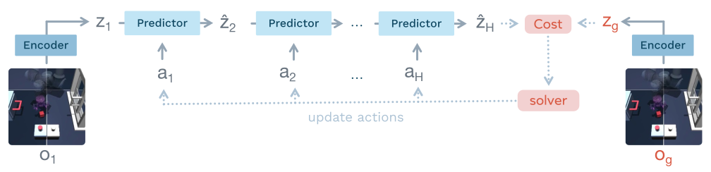
Figure 3 解读：latent planning 不需要 decoder，也不在像素空间比较预测图像。CEM 只需要反复调用 predictor，把候选动作序列 rollout 到 terminal latent，再比较 terminal latent 与 goal image 的 latent。这样 LeWM 的优势来自 compact representation：每帧只有一个 $192$ 维 token，而 DINO-WM 需要约 $200$ 倍更多视觉 tokens，因此同样的 planning 预算下 LeWM 可以更快评估 candidate plans。

def lewm_latent_cost(model, info, action_candidates, history_size=3):
    # info contains current pixels and goal image; action_candidates: (B, S, H, A)
    goal = {k: v[:, 0] for k, v in info.items() if torch.is_tensor(v)}
    goal["pixels"] = goal["goal"]
    goal.pop("action", None)
    goal_emb = model.encode(goal)["emb"]
 
    info = model.rollout(info, action_candidates, history_size=history_size)
    pred_emb = info["predicted_emb"]
    goal_emb = goal_emb[..., -1:, :].expand_as(pred_emb)
    cost = F.mse_loss(pred_emb[..., -1:, :], goal_emb[..., -1:, :].detach(), reduction="none")
    return cost.sum(dim=tuple(range(2, pred_emb.ndim)))

def cem_plan(model, info, horizon=5, num_samples=300, topk=30, iters=30):
    mean = torch.zeros(info["pixels"].size(0), horizon, info["action_dim"], device=info["pixels"].device)
    std = torch.ones_like(mean)
    for _ in range(iters):
        eps = torch.randn(mean.size(0), num_samples, *mean.shape[1:], device=mean.device)
        candidates = mean[:, None] + std[:, None] * eps
        scores = lewm_latent_cost(model, info, candidates)
        elite = candidates.gather(1, scores.topk(topk, largest=False).indices[..., None, None].expand(-1, -1, horizon, mean.size(-1)))
        mean = elite.mean(dim=1)
        std = elite.std(dim=1).clamp_min(1e-3)
    return mean

3.6 Code-to-paper mapping

Code reference: main @ c8a44170 (2026-05-17) — pseudocode and mapping based on this commit

Paper Concept	Source File	Key Class/Function
JEPA wrapper: encode pixels, predict next latent, planning cost	jepa.py	JEPA.encode, JEPA.predict, JEPA.rollout, JEPA.criterion, JEPA.get_cost
SIGReg anti-collapse regularizer	module.py	SIGReg.__init__, SIGReg.forward
Action-conditioned autoregressive predictor	module.py	ARPredictor, Transformer, ConditionalBlock
End-to-end training loss	train.py	lejepa_forward
Training hyperparameters	config/train/lewm.yaml	trainer, loader, optimizer, wm, loss.sigreg
Model architecture config	config/train/model/lewm.yaml	ViT-Tiny encoder, ARPredictor, action Embedder, projector / pred_proj MLPs
Dataset selection	config/train/data/*.yaml	pusht.yaml, tworoom.yaml, dmc.yaml, ogb.yaml
Evaluation / CEM planning configs	config/eval/*.yaml	plan_config, eval, dataset, world

4. Experimental Setup (实验设置)

4.1 Datasets and environments

论文覆盖四个 continuous action environments。TwoRoom 是 2D navigation，10,000 episodes，平均 trajectory length $92$，用 noisy heuristic policy 从一个房间穿过门到另一个房间目标点；PushT 是 2D manipulation，使用 DINO-WM 相同设定，20,000 expert episodes，平均长度 $196$，目标是推动 T-shaped block 到目标配置；OGBench-Cube 是 3D robotic manipulation，只考虑 single-cube variant，10,000 episodes，每个 episode $200$ steps，由 benchmark heuristic 生成；Reacher 来自 DeepMind Control Suite，10,000 episodes，每个 $200$ steps，用 Soft Actor-Critic policy 收集，目标是 2-joint arm 到达目标配置。所有环境都有 continuous action space。

Figure 4 解读：这张图说明 LeWM 不是只在一个 toy task 上验证。TwoRoom 低维且简单，PushT 需要物体交互，OGBench-Cube 增加 3D 视觉复杂度和机械臂，Reacher 则考察连续控制。后面的结果也显示 LeWM 的强项主要出现在更需要视觉-动作 dynamics 的 PushT / Reacher，而不是 intrinsic dimension 极低的 TwoRoom。

4.2 Baselines and metrics

主要 baselines 包括 DINO-WM、PLDM、GCBC、GCIQL、GCIVL、Random，有些图还报告 DINO-WM+proprio。DINO-WM 是 foundation-based latent world model，使用 DINOv2 features 来避免 collapse；PLDM 是最接近 LeWM 的 end-to-end pixel JEPA baseline，但 objective 包含多项 VICReg-derived losses；GCBC 是 goal-conditioned behavioral cloning；GCIQL 和 GCIVL 是 goal-conditioned offline RL。论文默认为了公平不让 DINO-WM 使用 proprioception，除非图中显式标注 DINO-WM+prop。

控制任务的主指标是 Success Rate (SR, 越高越好)，每个方法在目标条件下规划或执行后统计成功比例。Physical latent probing 使用 linear / MLP probe 从 latent embedding 预测物理量，报告 MSE (越低越好) 和 Pearson correlation $r$ (越高越好)。Violation-of-expectation 使用 surprise signal 比较 unperturbed、visual perturbation 与 physical perturbation 轨迹；如果模型真正学到物理连续性，那么 teleportation 这类违反物理的事件应比单纯颜色变化产生更高 surprise。

4.3 Training and evaluation config

论文 appendix 给出的训练细节是：frame-skip $5$；sub-trajectory size $4$，对应 $4$ frames 和 $4$ blocks of $5$ actions；输入 frame 分辨率 $224\times 224$；batch size $128$；每个 world model 在各数据集上训练 $10$ epochs；训练和 planning 均在单张 NVIDIA L40S GPU 上完成。模型约 $15$M 参数，其中 ViT-Tiny encoder 约 $5$M，predictor 约 $10$M。planning 设置为 CEM，每步 $300$ candidates，top $30$ elites，PushT 最多 $30$ iterations，其他环境 $10$ iterations，horizon $5$ latent steps / $25$ environment timesteps。

released config 中需要注意两个复现点：config/train/lewm.yaml 设置 batch_size: 128、img_size: 224、optimizer: AdamW、lr: 5e-5、weight_decay: 1e-3、precision: bf16、gradient_clip_val: 1.0、history_size: 3、num_preds: 1、embed_dim: 192、loss.sigreg.weight: 0.09、knots: 17、num_proj: 1024。同一文件的 trainer.max_epochs: 100 是 released Hydra 默认配置；论文实验文字明确写各环境 world model 训练 $10$ epochs，因此不能把该 default 直接当作论文主实验训练轮数，除非具体 launch 覆盖没有公开。

5. Experimental Results (实验结果)

5.1 Planning efficiency and control performance

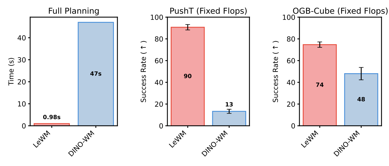
Figure 5 解读：左图给出 full planning wall-clock time：LeWM 为 $0.98$s，DINO-WM 为 $47$s，约 $48\times$ speedup。中、右图在 fixed FLOPs 下比较规划成功率：PushT 上 LeWM 为 $90$，DINO-WM 为 $13$；OGBench-Cube 上 LeWM 为 $74$，DINO-WM 为 $48$。这说明 LeWM 的优势不只是“模型小”，而是在同等计算预算内可以评估更多或更有效的 latent rollouts。

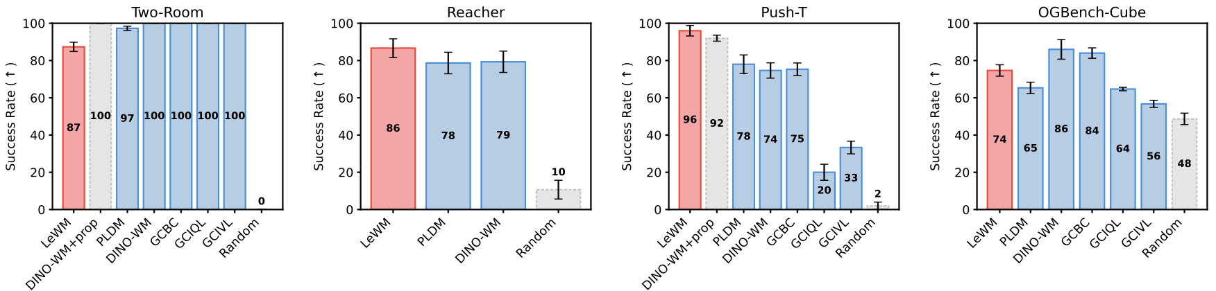
Figure 6 解读：四个环境的 SR 数字揭示了 LeWM 的边界。TwoRoom 上 LeWM 为 $87$，低于 DINO-WM+prop $100$、PLDM $97$、DINO-WM $100$ 以及 goal-conditioned baselines；作者解释为 TwoRoom intrinsic dimension 太低，SIGReg 在高维 Gaussian latent 中可能反而不利于结构化。Reacher 上 LeWM 为 $86$，超过 PLDM $78$、DINO-WM $79$ 和 Random $10$。PushT 上 LeWM 为 $96$，高于 DINO-WM+prop $92$、PLDM $78$、DINO-WM $74$、GCBC $75$、GCIQL $20$、GCIVL $33$、Random $2$。OGBench-Cube 上 LeWM 为 $74$，超过 PLDM $65$、GCIQL $64$、GCIVL $56$、Random $48$，但低于 DINO-WM $86$ 和 GCBC $84$；作者认为 3D visual complexity 使从零训练 encoder 更困难，而 DINOv2 pretraining 给 DINO-WM 带来优势。

综合看，LeWM 最强的 evidence 是 PushT 与 Reacher：它在没有 proprioception、没有 reward、没有 pretrained encoder 的情况下，仍超过 PLDM 和 DINO-WM 的 pixel-only setting。OGBench-Cube 暴露了端到端小模型在复杂 3D perception 上的限制；TwoRoom 暴露了 SIGReg 对 very low-dimensional dynamics 的 mismatch 风险。因此论文结论不是“LeWM everywhere best”，而是“端到端 pixel JEPA 可以稳定训练，并在多个非平凡控制任务中用更少计算达到竞争性或更好规划结果”。

5.2 Latent physical structure

PushT probing 结果表明，LeWM latent 中可以恢复 agent location、block location 和 block angle 等物理量。部分精确数字如下：

Property	Model	Linear MSE↓	Linear r↑	MLP MSE↓	MLP r↑
Agent Location	DINO-WM	$1.888\pm 0.500$	$0.977$	$0.003\pm 0.022$	$0.999$
Agent Location	PLDM	$0.090\pm 0.311$	$0.955$	$0.014\pm 0.119$	$0.993$
Agent Location	LeWM	$0.052\pm 0.149$	$0.974$	$0.004\pm 0.056$	$0.998$
Block Location	DINO-WM	$0.006\pm 0.007$	$0.997$	$0.002\pm 0.003$	$0.999$
Block Location	PLDM	$0.122\pm 0.341$	$0.938$	$0.011\pm 0.066$	$0.994$
Block Location	LeWM	$0.029\pm 0.073$	$0.986$	$0.001\pm 0.006$	$0.999$
Block Angle	DINO-WM	$0.050\pm 0.101$	$0.979$	$0.009\pm 0.052$	$0.995$
Block Angle	PLDM	$0.446\pm 0.625$	$0.745$	$0.056\pm 0.184$	$0.972$
Block Angle	LeWM	$0.187\pm 0.359$	$0.902$	$0.021\pm 0.139$	$0.990$

这张表的含义是：LeWM 明显强于 PLDM，尤其是 block location / angle；DINO-WM 在一些 MLP probe 上仍很强，作者认为这可能来自 DINOv2 在约 $124$M images 上预训练带来的默认视觉 prior。LeWM 的价值是用小得多、端到端的任务轨迹训练，在关键物理量上接近 foundation encoder 的可探测性。

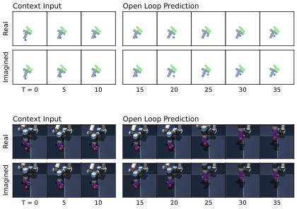
Figure 7 解读：这组 decoded rollout 不是训练目标，而是验证 latent prediction 是否真的保留场景 dynamics。PushT 中 imagined trajectory 能跟随真实 agent / block motion；OGBench-Cube 中大体场景布局和 cube displacement 保留，但 end-effector orientation 等细节会在长 horizon 上变差，这与 OGBench-Cube probing 中 rotation / fine-grained 量较难恢复一致。

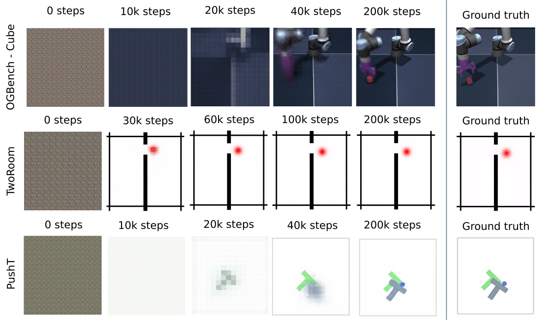
Figure 8 解读：decoder visualization 显示即使训练时没有 reconstruction loss，随着训练推进，单个 $192$ 维 [CLS] latent 仍能让外部 decoder 重建出主要场景结构。早期 decoded image 更像 slow features，后期逐渐包含任务相关物体与位置。这支持论文观点：LeWM 不需要像素重建目标，也可以在 latent 中保留足够的物理状态信息。

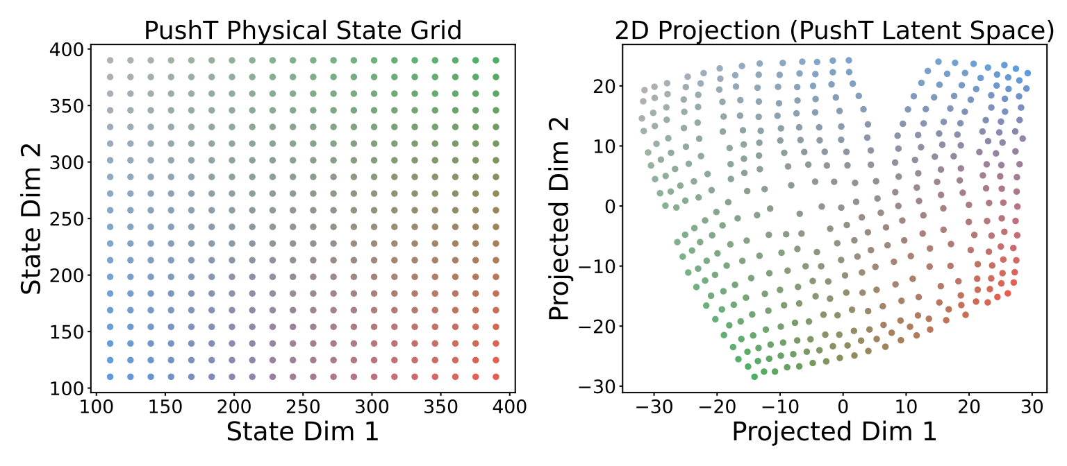
Figure 9 解读：PushT latent 的 t-SNE 可视化显示，移动 agent 和 block 得到的状态网格在 embedding space 中保留邻近关系。它不是严格定量证明，但提供了直观证据：SIGReg 并没有把所有状态随机打散，而是允许 spatial structure 在 Gaussian-like latent 中形成连续组织。

5.3 Violation-of-expectation and surprise

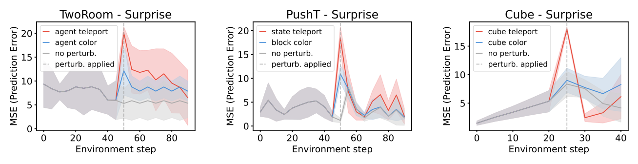
Figure 10 解读：VoE 实验比较三类轨迹：unperturbed、visual perturbation（物体颜色突变）和 physical perturbation（物体或 agent 被 teleport）。LeWM 对 teleportation 在 TwoRoom、PushT、OGBench-Cube 上都产生显著 surprise spike，paired t-test $p<0.01$；而 cube color perturbation 的 increase 更弱且不显著。这个结果说明 LeWM 的 surprise 更敏感于物理连续性被破坏，而不是简单把所有视觉变化都当成同等异常。

5.4 Ablations and stability

训练稳定性方面，PushT 三个 seed 的 SR 为 DINO-WM $92.0\pm 1.63$、PLDM $78.0\pm 5.0$、LeWM $96.0\pm 2.83$。PLDM variance 更高，LeWM 在高成功率下保持较低方差。predictor size ablation 显示 ViT-S 最好：tiny $80.67\pm 6.54$、small $96.0\pm 2.83$、base $86.7\pm 3.06$。加入 decoder reconstruction loss 反而从 $96.0\pm 2.83$ 降到 $86.0\pm 7.54$，支持“不重建像素也足够控制”的主张。encoder architecture 上，LeWM ViT 为 $96.0\pm 2.83$，ResNet-18 为 $94.0\pm 3.27$，说明方法不完全依赖某个特定视觉 backbone。predictor dropout 上，$p=0.1$ 最好：$p=0.0$ 为 $78\pm 6.54$，$p=0.1$ 为 $96.0\pm 2.83$，$p=0.2$ 为 $85.33\pm 5.74$，$p=0.5$ 为 $66.67\pm 4.11$。

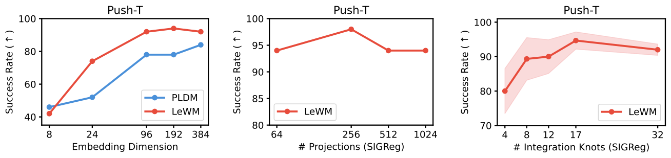
Figure 11 解读：embedding dimension 太小时性能下降，但超过约 $184$ 后收益饱和；SIGReg 的 projection 数 $M$ 和 integration knots 对结果不敏感。这个组合支持论文的调参论点：SIGReg 内部数值近似参数不需要精细调，真正需要搜索的是 $\lambda$。

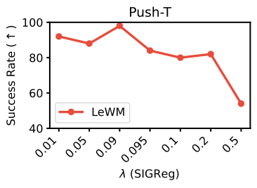
Figure 12 解读：$\lambda \in [0.01,0.2]$ 时 PushT SR 都保持在 $80\%$ 以上，峰值接近 $0.09$；当 $\lambda =0.5$ 时性能急剧下降，说明 regularizer 过强会压过 dynamics prediction，使表示更像“为了高斯而高斯”，不再服务于控制。

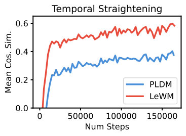
Figure 13 解读：LeWM 的 latent trajectory 在训练中出现 temporal straightening，即连续 latent velocity 的 cosine similarity 上升。PLDM 有显式 temporal smoothness regularization，但 LeWM 在没有此项 loss 的情况下出现更强 straightening。作者推测原因是 SIGReg 逐时间步施加而不显式约束时间维度，使 encoder 形成一种有利于控制的“时间上更线性”的隐式偏置。

5.5 Limitations and takeaways

作者明确承认 LeWM 仍有边界：第一，TwoRoom 这种低 intrinsic-dimensionality 环境中，高维 isotropic Gaussian prior 可能与真实状态流形不匹配，导致 LeWM 不如 PLDM / DINO-WM / goal-conditioned baselines。第二，在 OGBench-Cube 这种视觉复杂 3D 任务上，DINO-WM 由于 DINOv2 pretraining 仍领先，说明从零端到端训练小 encoder 在复杂视觉 priors 上有成本。第三，decoded rollout 中 finer details 如 end-effector orientation 会随 horizon 变差，auto-regressive latent rollout 仍有误差累积问题。第四，released code 主要依赖 stable-worldmodel 与 stable-pretraining 框架，论文主 repo 保留核心模型与 loss；复现完整数据、planner wrapper 和 baseline 仍需跟随这些外部库与 Hugging Face 数据/checkpoints。

总体结论是：LeWM 把端到端 JEPA world model 的稳定训练问题压缩为一个非常小的机制组合——prediction loss 学 dynamics，SIGReg 防 collapse，CEM 在 compact latent 中做 goal matching。它不是所有 benchmark 的 SOTA，但它证明了一个重要方向：无需 frozen foundation encoder 和复杂多 loss，raw-pixel JEPA 也可以训练出能规划、能探测物理变量、能对物理违例产生 surprise 的 latent world model。