Hierarchical Planning with Latent World Models

Paper: arXiv:2604.03208 Code: kevinghst/HWM_PLDM Code reference: main @ e197375b (2026-04-06)

1. Motivation（研究动机）

当前基于 learned world model 的 MPC 在 embodied control 中有一个很诱人的优点：模型可以只从 reward-free / task-agnostic offline trajectories 学 dynamics，然后在新任务上通过 goal-conditioned planning 零样本部署，不必为每个任务重新训练 policy。问题是这种范式一进入 long-horizon control 就暴露两个根本瓶颈。

第一，world model 的 rollout 会累积误差。低层模型通常擅长一步或短窗口预测，但如果为了到达远处 goal 必须 autoregressively rollout 很多步，小的 latent prediction error 会不断放大，最后 planner 优化的是不可靠的未来。第二，即使 dynamics 是完美的，直接在 primitive action sequence 上做长 horizon search 也会遇到组合爆炸：horizon 越长，CEM / MPPI 需要探索的 action sequence 空间越大，固定 compute budget 下很容易只找到 greedy 或局部可行的动作。

这篇论文要解决的具体问题不是“再训练一个更大的 policy”，而是：怎样在已经学好的 latent world models 上，把 long-horizon reasoning 和 short-horizon execution 分开，让 zero-shot MPC 能完成非 greedy、多阶段的机器人任务和导航任务。 这件事重要，因为一旦成功，world model 就可以成为通用 planner：高层负责找可解释的 latent subgoals，低层负责执行精细动作，系统不需要人工给中间目标，也不需要任务特定的 skill / option policy。

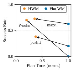
Figure 1 解读：这张总览图把论文的主要动机和结论放在一起。上半部分展示 high-level planner 在 latent space 里用 macro-actions 朝最终 goal 搜索，得到的第一个预测 latent state 被低层当作 subgoal；底部的实验覆盖图说明 hierarchy 在 Franka、Push-T、Diverse Maze 等不同 world model / task 上都能带来增益；右下角的 compute curve 强调 HWM 不是单纯用更多 search 换性能，而是在更低 planning time 下达到相近或更高 success。

2. Idea（核心思想）

核心 insight 是：hierarchy 不一定要靠学一个 hierarchical policy 或显式 skill library；如果多个 temporal scale 的 world model 共享 latent representation，那么高层预测出的未来 latent state 本身就可以作为低层 MPC 的 subgoal。 这样，高层只需要在抽象 latent action 空间里做长程搜索，低层只需要在 primitive action 空间里解决短程可达性。

HWM 的关键创新是把 temporal abstraction 放在 inference-time planning 中：低层 world model $P^{(1)}$ 学 primitive action dynamics，高层 world model $P^{(2)}$ 学由 action encoder 压缩出的 macro-action dynamics；规划时先最小化最终 goal latent 的高层 energy，再把第一个高层预测 latent 交给低层 MPC。

它和传统 hierarchical RL / options 的根本差别在于：HWM 不训练任务特定 high-level policy，也不要求低层 skill policy 接受 symbolic subgoal；相比 flat VJEPA2-AC / DINO-WM / PLDM planner，HWM 改变的是 planner 的 temporal structure，而不是低层模型的训练目标。论文实验也刻意复用底层 world model recipe，以隔离“hierarchical planning 本身”的贡献。

3. Method（方法）

3.1 总体框架：top-down latent-space MPC

给定当前 observation $s_1$ 和 goal observation $s_g$，共享 encoder $E$ 把它们映射到 latent states： $z_1=E(s_1),z_g=E(s_g).$ HWM 假设有两个时间尺度的 latent world model： $P^{(1)}(z_{t+1}\mid z_t,a_t),P^{(2)}(z_{t+h}\mid z_t,l_t).$ 其中 $a_t$ 是 primitive action，$l_t$ 是由 action encoder $A_{\psi }$ 从一段低层动作压缩得到的 latent macro-action。规划过程是 top-down 的：高层先搜索 $H$ 个 latent actions，使预测轨迹靠近最终 goal；然后低层只追踪高层轨迹中的第一个 subgoal，并按 receding-horizon MPC 不断重规划。

高层 energy 写作： ${\mathcal{E}}_2({\hat{l}}_{1:H};z_1,z_g)={\Vert z_g-P^{(2)}({\hat{l}}_{1:H};z_1)\Vert }_1,$ $l_{1:H}^{\ast }=\arg {\min }_{{\hat{l}}_{1:H}}{\mathcal{E}}_2({\hat{l}}_{1:H};z_1,z_g).$ 展开最优 latent plan 得到高层子目标： ${\tilde{z}}_i=P^{(2)}(l_{1:i}^{\ast };z_1),i=1,\dots ,H.$ 低层只追踪第一个 latent subgoal： ${\mathcal{E}}_1({\hat{a}}_{1:h};z_1,{\tilde{z}}_1)={\Vert {\tilde{z}}_1-P^{(1)}({\hat{a}}_{1:h};z_1)\Vert }_1,$ $a_{1:h}^{\ast }=\arg {\min }_{{\hat{a}}_{1:h}}{\mathcal{E}}_1({\hat{a}}_{1:h};z_1,{\tilde{z}}_1).$ 直觉上，高层避免了“直接搜索一长串 primitive actions”的组合爆炸，低层避免了“长时间 rollout 一个短 horizon 模型”的误差累积。更重要的是，高层 subgoal 仍然是同一个 latent space 里的 state，不需要 inverse model 把 symbolic goal 翻译成 action，也不需要人工标注 skill boundary。

3.2 低层 latent world model：复用已有短程 dynamics

低层模型 $P_{\theta }^{(1)}$ 预测短程 latent transition。论文没有为 HWM 重新设计低层模型，而是分别复用对应 benchmark 的原始 world model recipe：Franka 使用 VJEPA2-AC，Push-T 使用 DINO-WM，Diverse Maze 使用 PLDM。训练目标包含 teacher forcing 和多步 autoregressive rollout loss： ${\hat{z}}_{k+1}=P_{\theta }^{(1)}((a_t,z_t{)}_{t\le k}),{\mathcal{L}}_{\mathrm{tf}}(\theta )=\frac{1}{T}{\sum }_{k=1}^T\Vert {\hat{z}}_{k+1}-z_{k+1}{\Vert }_1.$ 多步 rollout loss 用 $P_{\theta }^{(1)}(a_{1:j};z_1)$ 表示从 $z_1$ 开始按动作序列 autoregressive 得到的最终 latent： ${\mathcal{L}}_{\mathrm{roll}}(\theta )={\sum }_{j=2}^T{\Vert P_{\theta }^{(1)}(a_{1:j};z_1)-z_{j+1}\Vert }_1,$ $\mathcal{L}(\theta )={\gamma }_{\mathrm{tf}}{\mathcal{L}}_{\mathrm{tf}}(\theta )+{\gamma }_{\mathrm{roll}}{\mathcal{L}}_{\mathrm{roll}}(\theta ).$ 论文的实验设计强调：低层模型不因为 HWM 而换 architecture，因此 Franka 上 VJEPA2-AC flat planner 与 HWM 的差异主要来自 hierarchy；Push-T 与 Diverse Maze 同理。

3.3 高层 latent world model 与 latent action encoder

高层模型 $P_{\varphi }^{(2)}$ 不是直接吃 primitive actions，而是吃 macro latent actions。给定轨迹 $\tau =(s_1,a_1,s_2,a_2,\dots ,s_T)$，先选择 waypoint indices $1=t_1<t_2<\cdots <t_N$。第 $k$ 个高层 transition 是： $\left(s_{t_k},a_{t_k:t_{k+1}},s_{t_{k+1}}\right).$ 共享 encoder 得到 waypoint latents $(z_{t_k})$，action encoder $A_{\psi }$ 把动作片段 $a_{t_k:t_{k+1}}$ 编成 macro-action $l_{t_k}$。高层 world model 接收交错的 $(l_{t_i},z_{t_i}{)}_{i\le k}$ 并预测下一个 waypoint latent： ${\hat{z}}_{t_{k+1}}:=P_{\varphi }^{(2)}\left((l_{t_i},z_{t_i}{)}_{i\le k}\right),$ ${\mathcal{L}}_{\mathrm{tf}}(\varphi ,\psi )=\frac{1}{N}{\sum }_{k=1}^N{\Vert {\hat{z}}_{t_{k+1}}-z_{t_{k+1}}\Vert }_1.$

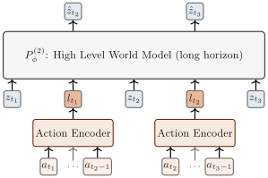
Figure 2 解读：高层训练图显示了 HWM 的关键接口：低层动作片段先被 action encoder 压缩成 $l_t$，再和 waypoint latent state 交错输入 causal high-level world model。高层模型预测的是未来 waypoint 的 latent representation，而不是像素或动作；这使它可以和低层 planner 直接通过 latent-state matching 连接。

不同任务的高层 action encoder 实例化不同：Franka 和 Push-T 使用 transformer-based action encoder，CLS token 经过 MLP head 得到 latent action；Diverse Maze 的 released code / appendix 使用 MLP 把 primitive action chunks 编成 8-dimensional latent action。Franka 高层 latent action dimension 在主实验中设为 4；Diverse Maze released config 中 large_diverse_25maps_l2.yaml 使用 z_dim: 8、l2_step_skip: 10、l2_n_steps: 6。

3.4 Planning：CEM / MPPI 的两层目标如何交互

Franka 和 Push-T 使用 CEM；Diverse Maze 使用 MPPI。两者共同点是：planner 采样 action sequences，用 learned dynamics rollout，按 latent target distance 计算 cost，然后执行优化序列的前几个动作并重规划。

论文给出的 CEM hyperparameters 很具体。单层 Franka 使用 2400 samples、15 iterations、20 elites、prediction horizon 6、$k=1$；HWM Franka 高层使用 3000 samples、15 iterations、22 elites、prediction horizon $H=2$，低层使用 800 samples、5 iterations、12 elites、prediction horizon $h=2$，每步重规划。Push-T 的 HWM 在 $d=25/50/75$ 上分别使用高层 samples $900/1500/1200$、高层 horizon $2/4/5$，低层 samples $300/900/1200$、低层 horizon 均为 5，$k=5$。

Diverse Maze 的 released config 走 MPPI：large_diverse_25maps_l2.yaml 中 medium/hard 难度高层分别使用 num_samples=2000/4000，论文 MPPI table 的 high-level prediction horizon 为 $H=35/47$；低层使用 num_samples=500/1000，论文 table 的 low-level prediction horizon 固定为 $h=15$，$k=4$。这里要区分两个量：released YAML 里的 max_plan_length=50 是 evaluation level 的 episode/planning cap，而不是论文 MPPI table 中的低层 pred $h$。代码中 TwoLvlPlanner.plan() 的实际接口很直接：先用 L1 backbone encode 当前状态，L2 planner 对最终 goal planning；然后把 l2_result.pred_obs[1] 设为 L1 planner 的 target，让 L1 在 l2_step_skip 个 primitive steps 内追踪它。

3.5 论文公式与 released code 实现差异

论文主文和 appendix 用 $L_1$ 形式描述低层/高层 teacher-forcing 与 rollout prediction loss；但 released PLDM implementation 中，pldm/objectives/prediction.py 的 PredictionObjective 对 PredictionObs / PredictionProprio 使用 (encodings - predictions).pow(2).mean()，即 MSE-style loss。Diverse Maze 的 released config pldm/configs/diverse_maze/icml/large_diverse_25maps_l2.yaml 也把高层 objectives 设为 PredictionObs 与 PredictionProprio，因此该开源实现的训练损失与论文公式的 $L_1$ 写法并不完全一致。

另一个边界是 release scope：GitHub repo 明确说它是 PLDM / Diverse Maze 的 minimal implementation；Franka 的 VJEPA2-AC 与 Push-T 的 DINO-WM 完整训练/evaluation pipeline 不在该 repo 中。因此本笔记中的 pseudocode 和 mapping 以 released PLDM code 为锚点，Franka / Push-T 的训练数值主要来自论文 appendix。

3.6 代码级伪代码：高层训练、两层规划、MPPI rollout

Code reference: main @ e197375b (2026-04-06) — pseudocode and mapping based on this commit

高层训练路径对应 pldm/models/hjepa.py + pldm/train.py + pldm/objectives/*.py。论文中 Franka / Push-T 使用 transformer-based action encoder；但 released PLDM / Diverse Maze code 是另一种实现：large_diverse_25maps_l2.yaml 固定 l2_step_skip=10、l2_n_steps=6，把 10 个 primitive 2D actions 拼成 posterior_input_dim=20 的 chunk，并在 level-2 predictor 中用 action_encoder_arch: '8-64-8' 的 MLP-style encoder 处理 8D latent action。因此下面 pseudocode 以 released PLDM code 为准：

import torch
from pldm.models.predictors.conv_predictors import Expander2D
 
def build_diverse_maze_l2_sample(dataset, episode_idx, start_idx,
                                 step_skip: int = 10, l2_n_steps: int = 6,
                                 stack_states: int = 1):
    # Mirrors D4RLDataset.__getitem__ for level-2 samples.
    # Code uses l2_n_steps_total = l2_n_steps * l2_step_skip + 1.
    total = l2_n_steps * step_skip + 1
    l2_states, l2_locations, primitive_actions, l2_vel, l2_pos = dataset._load_data_from_start_idx(
        episode_idx=episode_idx,
        start_idx=start_idx,
        length=total + stack_states - 1,
        skip_frame=step_skip,
    )
 
    # _load_data_from_start_idx subsamples states/locations/proprio with skip_frame,
    # but keeps the dense primitive action interval [start_idx, end_idx - 1].
    # With total=61 and step_skip=10, this becomes 6 chunks of 10 actions.
    chunks = primitive_actions.split(step_skip)
    l2_actions = torch.stack(chunks, dim=0)  # [l2_n_steps, step_skip, action_dim]
    return l2_states, l2_actions, l2_locations, l2_vel, l2_pos
 
def posterior_chunk_to_latent(sequence_predictor, actions, i):
    # Mirrors SequencePredictor: posterior_input_type='actions'.
    # DataLoader supplies actions[i] as [batch, chunk_size, action_dim].
    posterior_input = actions[i]
    if sequence_predictor.config.posterior_arch != "analytical":
        posterior_input = posterior_input.view(posterior_input.shape[0], -1)  # [B, 20]
    posterior_mu, posterior_var = sequence_predictor.posterior_model(posterior_input)
    return posterior_mu  # deterministic released config uses the posterior mean/mode
 
class ReleasedPLDMPredictorActionEncoder(torch.nn.Module):
    def __init__(self):
        super().__init__()
        # Separate path from posterior_arch='32-32': this mirrors action_encoder_arch='8-64-8'
        # used by the level-2 predictor to expand an 8D latent action during prediction/planning.
        self.action_encoder = torch.nn.Sequential(
            torch.nn.Linear(8, 64),
            torch.nn.ReLU(),
            torch.nn.Linear(64, 8),
            Expander2D(w=16, h=16),
        )

实际 HJEPA training step 可抽象为：

import torch
import torch.nn.functional as F
 
def train_hjepa_step(hjepa, batch, objectives_l1, objectives_l2, optimizer, train_l1=False):
    states = batch["states"].cuda()       # [T, B, C, H, W]
    actions = batch["actions"].cuda()     # primitive or chunked actions
    optional = {
        "proprio_pos": batch.get("proprio_pos"),
        "proprio_vel": batch.get("proprio_vel"),
        "locations": batch.get("locations"),
        "l2_states": batch.get("l2_states"),
        "l2_actions": batch.get("l2_actions"),
        "l2_proprio_pos": batch.get("l2_proprio_pos"),
        "l2_proprio_vel": batch.get("l2_proprio_vel"),
    }
 
    result = hjepa.forward_posterior(states, actions, **optional)
 
    losses = []
    if train_l1:
        losses += [obj(batch, [result.level1]).total_loss for obj in objectives_l1]
    if result.level2 is not None:
        losses += [obj(batch, [result.level1, result.level2]).total_loss
                   for obj in objectives_l2]
 
    loss = sum(losses)
    optimizer.zero_grad()
    loss.backward()
    optimizer.step()
    return loss.detach()

两层 planner 对应 pldm/planning/planners/two_lvl_planner.py：

def hierarchical_plan_step(two_lvl_planner, current_obs, final_goal_repr,
                           curr_proprio_pos=None, curr_proprio_vel=None):
    two_lvl_planner.reset_targets(final_goal_repr, repr_input=True)
 
    l1_backbone_output = two_lvl_planner.l1_planner.model.backbone(
        current_obs.cuda(),
        proprio=torch.cat([curr_proprio_pos, curr_proprio_vel], dim=-1).cuda()
        if curr_proprio_pos is not None and curr_proprio_vel is not None else None,
    )
 
    l2_result = two_lvl_planner.l2_planner.plan(
        current_state=l1_backbone_output,
        plan_size=two_lvl_planner.l2_step_skip,
        repr_input=True,
    )
 
    next_latent_subgoal = l2_result.pred_obs[1].detach()
    two_lvl_planner.l1_planner.reset_targets(next_latent_subgoal, repr_input=True)
    l1_result = two_lvl_planner.l1_planner.plan(
        current_state=l1_backbone_output,
        plan_size=two_lvl_planner.l2_step_skip,
        repr_input=True,
        curr_proprio_pos=curr_proprio_pos,
        curr_proprio_vel=curr_proprio_vel,
    )
    return l1_result.actions, l2_result

Diverse Maze 的 MPPI planning 对应 pldm/planning/planners/mppi_planner.py 与 pldm/planning/planners/mppi_torch.py：

def mppi_command(model, state, target_repr, nominal_actions, noise_dist, objective,
                 num_samples: int, horizon: int, temperature: float):
    sampled_noise = noise_dist.sample((horizon, num_samples))
    action_sequences = nominal_actions[:, None, :] + sampled_noise
    costs = torch.zeros(num_samples, device=state.device)
 
    rollout_state = state.repeat(num_samples, *([1] * (state.ndim - 1)))
    for t in range(horizon):
        action_t = action_sequences[t]
        pred = model.forward_prior_or_posterior(rollout_state, action_t)
        rollout_state = pred.obs_component
        costs = costs + objective(rollout_state, target_repr)
 
    beta = costs.min()
    weights = torch.exp(-(costs - beta) / temperature)
    weights = weights / weights.sum().clamp_min(1e-8)
    updated_sequence = (weights[None, :, None] * action_sequences).sum(dim=1)
    return updated_sequence[0], updated_sequence

3.7 Code-to-paper mapping

Code reference: main @ e197375b (2026-04-06) — pseudocode and mapping based on this commit

Paper Concept	Source File	Key Class/Function
Two-level JEPA / HJEPA model	pldm/models/hjepa.py	HJEPA, HJEPAConfig, forward_posterior()
Low/high-level JEPA predictor	pldm/models/jepa.py; pldm/models/predictors/*	JEPA, predictor modules
Training loop and objective aggregation	pldm/train.py	Trainer.train(), model.forward_posterior(), objectives list
Prediction / VICReg objectives	pldm/objectives/prediction.py; pldm/objectives/vicreg.py; pldm/objectives/__init__.py	PredictionObjective, VICRegObjective, ObjectivesConfig.build_objectives_list()
Hierarchical planner interface	pldm/planning/planners/two_lvl_planner.py	TwoLvlPlanner.plan()
Planner construction and target encoding	pldm/planning/mpc.py; pldm/planning/d4rl/hmpc.py	_construct_h_planner(), _construct_planner(), HierarchicalD4RLMPCEvaluator
Representation target cost	pldm/planning/objectives_v2.py	ReprTargetMPCObjective, ReprTargetMPCObjective2
MPPI trajectory optimizer	pldm/planning/planners/mppi_planner.py; pldm/planning/planners/mppi_torch.py	MPPIPlanner, MPPI.command()
Released Diverse Maze configs	pldm/configs/diverse_maze/icml/large_diverse_25maps.yaml; large_diverse_25maps_l2.yaml	low-level / high-level PLDM hyperparameters

4. Experimental Setup（实验设置）

4.1 Datasets and tasks

• Franka Arm with Robotiq gripper：训练数据为约 96 小时 DROID unlabeled robot videos 与 30 小时 RoboSet；observation 包含 RGB image 与 7D end-effector proprioception，action 是 end-effector delta pose。评测包含 10 个 pick-and-place start-goal pairs（cup / box 两类物体）与 7 个 drawer opening / closing tasks。
• Push-T：使用 DINO-WM released offline dataset，共 18,500 trajectories；每条轨迹包含 RGB observation、2D action 与 agent position/velocity proprioception。评测把 start-goal separation 扩展到 $d=25,50,75$ timesteps，其中 $d=75$ 明显超过原 DINO-WM 的 $d=25$ 设置。
• Diverse Maze：MuJoCo PointMaze 变体，模型输入是 $(98,98,3)$ top-down RGB maze view，而不是直接使用 $(x,y)$。训练使用 25 个随机地图，每个地图 2,000 episodes，每个 episode 100 steps、action repeat 4，总计约 5M transitions；测试在 20 个 held-out layouts 上 zero-shot，按 grid distance 分 easy $D\in [5,8]$、medium $D\in [9,12]$、hard $D\in [13,16]$。

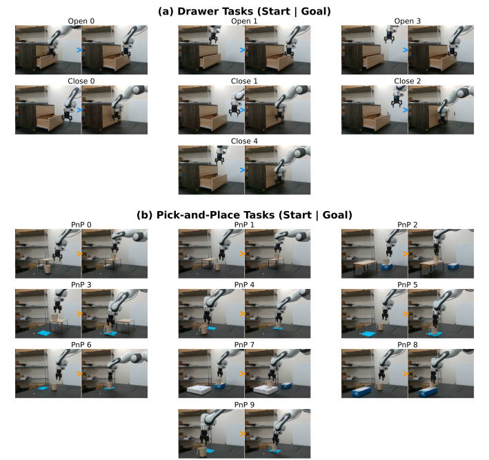
Figure 3 解读：这张 appendix 图列出了 evaluation tasks 的 initial / goal states。它有助于理解为什么这些任务不是简单 greedy reaching：drawer 和 pick-and-place 往往需要先移动到中间姿态，Push-T 与 Maze 也要求在远距离 start-goal pair 之间完成多阶段路径。

4.2 Baselines and metrics

Franka 对比 VJEPA2-AC flat planner，以及 Octo、${\pi }_0$-FAST-DROID、${\pi }_{0.5}$-DROID 三个 VLA baselines。Push-T 对比 GCIQL、HIQL、HILP 与 DINO-WM。Diverse Maze 对比 GCIQL、HIQL、HILP 与 PLDM。

主要 metric 是 success rate。分析部分还使用 planning time / normalized test-time compute、latent prediction $L_1$ error、high-level action 与 expert trajectory 的 action cosine similarity / action $L_1$ distance。Franka / Push-T 使用 CEM planning，Diverse Maze 使用 MPPI planning。

4.3 Training and planning configs

Franka：低层 VJEPA2-AC 使用 frozen ViT-g/16 encoder 与约 300M-parameter ViT world model，context $T=16$，epochs 200，batch size 256，${\gamma }_{\mathrm{tf}}=1.0$、${\gamma }_{\mathrm{roll}}=1.0$；高层 VJEPA2-AC context $T=3$，epochs 120，batch size 768，${\gamma }_{\mathrm{tf}}=1.0$、${\gamma }_{\mathrm{roll}}=0.0$。论文没有给出 GPU 型号/数量，只说明 planning rollouts parallel across GPUs。

Push-T：低层 DINO-WM 使用 frozen DINOv2 encoder 与 25M-parameter causal ViT，context $T=4$，epochs 100，batch size 256；高层 DINO-WM 扩到 75M parameters（layers 6→10，embedding 384→768，MLP 2048→3072，heads 16→12），context $T=5$，epochs 500，batch size 128。两者 ${\gamma }_{\mathrm{tf}}=1.0$、${\gamma }_{\mathrm{roll}}=0.0$。

Diverse Maze：论文 appendix 与 released config 对齐。低层 PLDM：pldm/configs/diverse_maze/icml/large_diverse_25maps.yaml，n_steps=15、batch size 128、epochs 3、base LR 0.017632900482959527、VICReg / IDM / proprio prediction objectives、planning n_envs=85、replan_every=4。高层 PLDM：pldm/configs/diverse_maze/icml/large_diverse_25maps_l2.yaml，l2_step_skip=10、l2_n_steps=6、batch size 128、epochs 5、freeze_l1=true、z_dim=8、PredictionObs + PredictionProprio objectives，加载低层 checkpoint 3-9-1-seed248_epoch=3_sample_step=15465472.ckpt。

5. Experimental Results（实验结果）

5.1 Main results across three domains

Franka robotic manipulation

Method	P&P Subgoals Cup	P&P Subgoals Box	P&P Cup	P&P Box	Drawer
Octo	20%	10%	0%	0%	43%
${\pi }_0$-FAST-DROID	—	—	52%	18%	—
${\pi }_{0.5}$-DROID	—	—	68%	36%	—
VJEPA2-AC	80%	80%	0%	0%	30%
VJEPA2-AC (hierarchy)	80%	80%	70%	60%	70%

Flat VJEPA2-AC 在人工 subgoals 下能完成 cup/box 的 greedy subtasks（80% / 80%），但只给 final goal 时 pick-and-place 完全失败（0% / 0%），drawer 也只有 30%。HWM 在不提供人工 subgoal 的情况下达到 cup 70%、box 60%、drawer 70%，说明高层自动提出的 latent subgoals 确实替代了手工分解。

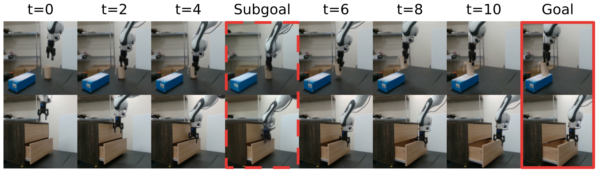
Figure 4a 解读：Franka execution strip 中红色虚线列表示高层 planner 推断并 decode 出来的 subgoal。可以看到 HWM 不是直接朝最终图像贪心移动，而是先到达抓取/对齐/抽屉操作等中间状态，再由低层短程 planner 执行。

Figure 4b 解读：Push-T execution 同样展示了 high-level subgoal 对 long-horizon pushing 的作用。T 形物体需要通过一系列中间位姿逼近 goal；flat planner 在 $d=75$ 时容易因为搜索 horizon 太长而失败，而 HWM 把问题拆成多个短程追踪。

Push-T long-horizon goal-conditioned control

Method	$d=25$	$d=50$	$d=75$
GCIQL	40%	25%	7.5%
HIQL	55%	30%	20%
HILP	25%	13%	0%
DINO-WM	84%	55%	17%
DINO-WM (hierarchy)	89%	78%	61%

Push-T 的关键趋势是 horizon 越长，flat DINO-WM 掉得越厉害：从 $d=25$ 的 84% 降到 $d=75$ 的 17%。HWM 在 $d=75$ 仍有 61%，绝对提升 44 个百分点。和 offline RL / zero-shot RL baselines 相比，HWM 的优势也随 horizon 扩大而更明显。

Diverse Maze OOD navigation

Method	$D\in [5,8]$	$D\in [9,12]$	$D\in [13,16]$
GCIQL	85%	40%	33%
HIQL	88%	73%	48%
HILP	48%	20%	10%
PLDM	100%	63%	44%
PLDM (hierarchy)	100%	95%	83%

Diverse Maze 说明 HWM 不只适用于机器人手臂，也适用于从像素输入做 latent planning 的 navigation。训练和测试地图 layout 不同，且 hard split 的距离达到 $D\in [13,16]$；PLDM flat planner 在 hard 上是 44%，加 hierarchy 后到 83%。

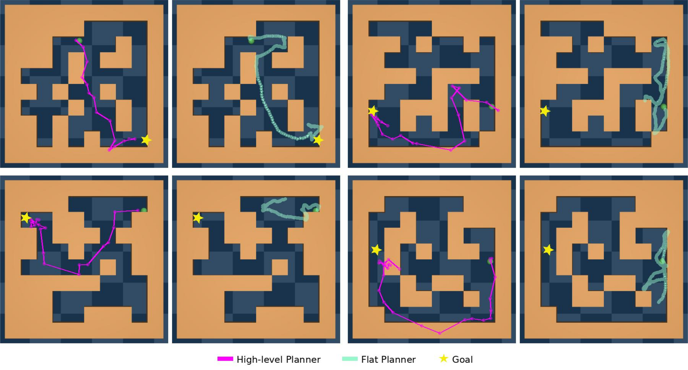
Figure 5 解读：Maze plans 图把高层 plan 和低层执行放在同一张图里。高层轨迹在较粗时间尺度上跨越长距离 maze corridor，低层 planner 负责局部转向和避墙；这正对应 HWM “长程抽象 + 短程控制”的分工。

5.2 Compute efficiency and long-horizon prediction

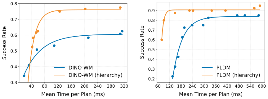
Figure 6 解读：左侧 Push-T、右侧 Diverse Maze 都画出 success rate 与 planning time 的 trade-off。论文结论是，HWM 在 Push-T 上可以用约 $3\times$ 更低 compute 达到或超过 flat planner，在 Diverse Maze 上则约 $4\times$ 更低 compute。原因不是高层模型更便宜，而是它显著缩短了低层 primitive action search 的有效 horizon。

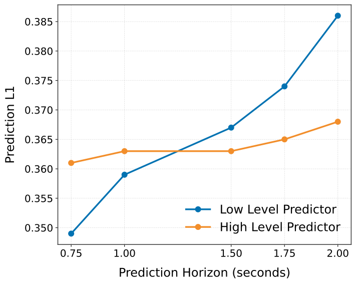
Figure 7 解读：prediction horizon 分析验证了 hierarchy 的另一个前提：低层 world model 在短 horizon（约 $<1$ 秒）更准，但要预测到 1.5–2 秒后时，高层单步 prediction 比低层多步 autoregressive rollout 的 $L_1$ error 更低。也就是说，高层不是替代低层，而是在低层误差开始累积的时间尺度上接管。

5.3 Ablations: latent actions and subgoal quality

High-Level Action	Action Cos $\uparrow$	Action L1 $\downarrow$
Delta Pose	$0.80\pm 0.02$	$0.088\pm 0.005$
Latent Action	$0.88\pm 0.03$	$0.080\pm 0.002$

这组 action alignment 结果说明 learned latent action 比直接用 delta-pose 更贴近 expert behavior：cosine similarity 更高、L1 distance 更低。论文的解释是，latent action encoder 可以压缩一段 primitive actions 中对高层 planning 有用的可控变化，而不是把所有低层细节都暴露给高层 optimizer。

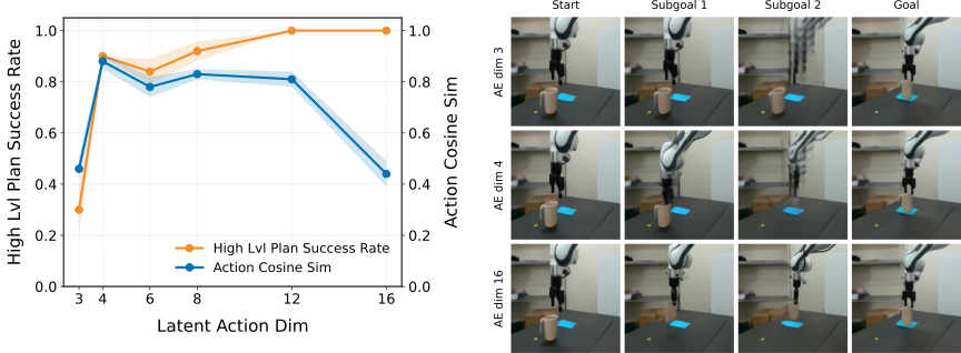
Figure 8 解读：latent action dimension 有一个 trade-off。维度太低时，高层模型容量不足，plan success 低；维度升高后，视觉重建和 plan 表达力改善，但过高维度也可能让高层提出低层难以 greedy 到达的 subgoal。Franka 上经验最优大约是 4D：足够表达 useful trajectories，但不会过度鼓励不可执行的 non-greedy subgoals。

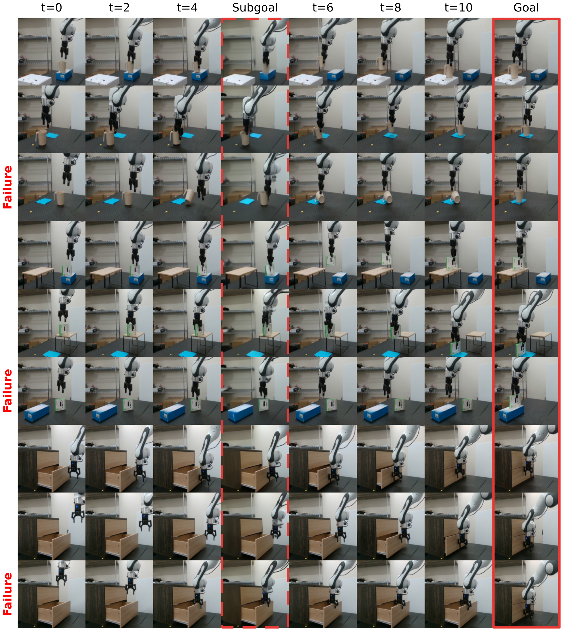
Figure 9 解读：appendix 的 thorough rollout 图补充了成功与失败案例。失败通常不是 hierarchy 完全失效，而是 perceptual imprecision、深度估计误差或接近目标但未精确完成；这对应作者在主文中提到的 limitation：长程 manipulation 仍然需要更抽象且 uncertainty-aware 的 representation / planning。

5.4 Limitations and conclusions

HWM 的主要结论是：hierarchical planning 是一种 model-agnostic extension，可以在 VJEPA2-AC、DINO-WM、PLDM 三类 latent world model 上提高 zero-shot long-horizon control，尤其在 flat planner 受限于 long rollout error 或 action search 空间时最明显。

限制也很清楚。第一，所有方法随着 horizon 增长仍会退化；HWM 缓解但没有消除 long-horizon manipulation 的难度。第二，高层 subgoal 是 strictly top-down 提供给低层，当前方法缺少跨层 feedback / joint optimization；如果高层提出“语义合理但低层不可达”的 subgoal，低层仍会失败。第三，论文认为未来需要更 abstract 的 high-level representation 与 uncertainty-aware planning，来处理真实世界长程预测中的 stochasticity 与 model uncertainty。