Recursive Flow Matching

Paper: arXiv:2605.26535 Project: jhhuangchloe.github.io/RecFM Code: 代码搜索未找到开源实现；官方占位仓库 Rose-STL-Lab/RecFM 仅含 Coming soon.，因此本笔记不设置 github_ref。

1. Motivation (研究动机)

当前科学系统 emulation 的核心矛盾是 speed-fidelity trade-off：传统数值求解器能给出高保真物理轨迹，但在流体、气候、声学散射等高维时空系统上成本高，难以用于实时预测或大规模 ensemble；Diffusion / video diffusion emulator 虽然能建模复杂分布和不确定性，却通常需要很多 sequential denoising steps，推理代价高，并且长 rollout 中容易累积误差。

Flow Matching (FM) 缓解了 diffusion 的训练模拟成本问题：它直接学习从 data distribution $p_{0}$ 到 noise distribution $p_{1}$ 的连续 velocity field。但 vanilla FM 在少步数推理时仍不稳定，因为训练只监督一条 linear probability path；当 Euler solver 用很大的 step size 走完整条 ODE 时，任何 trajectory curvature / discretization error 都会被放大。Shortcut / consistency / distillation 试图把多步生成压成一步，但在物理场上常见的问题是高频结构被抹平、spectral richness 下降，导致准确性和物理一致性下降。

这篇论文要解决的具体问题是：如何让 spatiotemporal physics generative emulator 在 1-step 或 few-step 推理下仍保持接近多步 SOTA solver 的预测精度、calibration 和物理一致性。这值得研究，因为一旦少步生成可行，就能把 diffusion-style scientific emulator 从离线模拟工具推进到实时/交互式 scientific emulation：例如快速流体预测、气候场 ensemble、声学波场 rollout，以及需要大量条件采样的 inverse design / uncertainty quantification。

2. Idea (核心思想)

RecFM 的核心洞察是：vanilla FM 只把同一个 $x_{t}$ 看成 primary trajectory 上的一个点，而 RecFM 让同一个 spatial point $x_{t}$ 同时落在多个 time-rescaled / scale-rescaled trajectories 上；这些轨迹的 velocity 应当按 scale $α$ 成比例一致。因此，模型不是只学一个 target velocity，而是在同一位置学习一族递归缩放的 velocity，并用 cross-scale consistency 把它们对齐。

关键创新可以概括为三点：第一，引入 wall-bouncing pendulum 的速度衰减直觉，把多尺度轨迹速度写成 $v^{(i)} = α^{(i)} v^{*}$ ；第二，把 velocity network 扩展为 $v_{θ} (x, t, α)$ ，显式 conditioning on scale；第三，在 trajectory supervision 外加入 consistency loss，使不同尺度的预测满足 $\overset{v}{^}^{(i)} \approx α^{(i)} \overset{v}{^}^{(1)}$ ，从而 straightening trajectory、降低少步 Euler 截断误差。

它与 Shortcut Diffusion / one-step consistency model 的本质差别在于：Shortcut 通常学习“同一轨迹上任意两点到同一 endpoint 的一致性”，更像 endpoint mapping 的自一致；RecFM 学的是 不同缩放轨迹在同一个 $x_{t}$ 处的 velocity 一致性，不需要先训练 teacher 或 warm-up 多步模型，也不把物理 rollout 简化为 endpoint regression，而是直接正则化 learned velocity field 的尺度结构。

3. Method (方法)

3.1 Overall framework：从单条 FM 轨迹扩展到递归多尺度轨迹

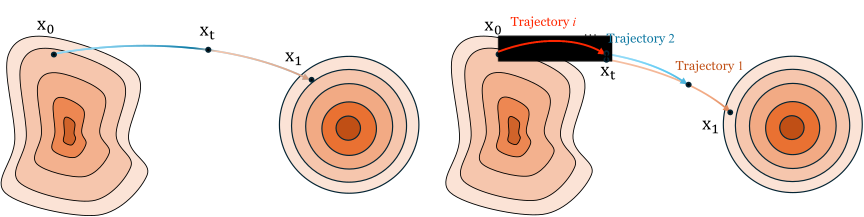
Figure 1 解读：左侧 vanilla Flow Matching 只学习从 $x_{0}$ 到 $x_{1}$ 的单条 direct trajectory；右侧 RecFM 在同一个 spatial state $x_{t}$ 处引入多条缩放轨迹，棕/蓝/红箭头表示不同 $α$ scale 下的 velocity。关键不是额外采样更多噪声，而是让一个 velocity network 在相同 $x_{t}$ 、不同 $(τ, α)$ conditioning 下输出成比例一致的速度，从训练时就约束少步推理会走的“大步轨迹”。

标准 FM 使用 linear interpolant： $x_{t} = (1 - t) x_{0} + t x_{1}, v^{*} = x_{1} - x_{0},$ 其中 $x_{0} \sim p_{0}$ 是 data sample， $x_{1} \sim p_{1}$ 是 noise sample。RecFM 保留这条 primary trajectory，但把 velocity network 写成： $v_{θ} (x, t, α), t \in [0, 1], α \in (0, 1] .$ 递归深度 $D$ 给出 $D$ 条 trajectory scale： $α^{(1)} = 1$ ，通常 $α^{(i)} = α^{i - 1}$ ；为了让这些轨迹穿过同一个 $x_{t}$ ，第 $i$ 条轨迹使用 rescaled time： $τ^{(i)} = \frac{t}{α ^{(i)}} \in [0, 1], \overset{v}{^}^{(i)} = v_{θ} (x_{t}, τ^{(i)}, α^{(i)}) .$ 直观上，RecFM 把“同一个训练点”变成多个 supervision views：primary view 学 $x_{1} - x_{0}$ ，secondary views 学 $α^{(i)} (x_{1} - x_{0})$ 。这相当于在 conditioning space 上做 data augmentation，但它不是任意增广；所有 targets 都由同一条 OT direction 派生，因此能稳定约束 velocity field 的 local geometry。

3.2 Physics intuition：wall-bouncing pendulum 的速度缩放

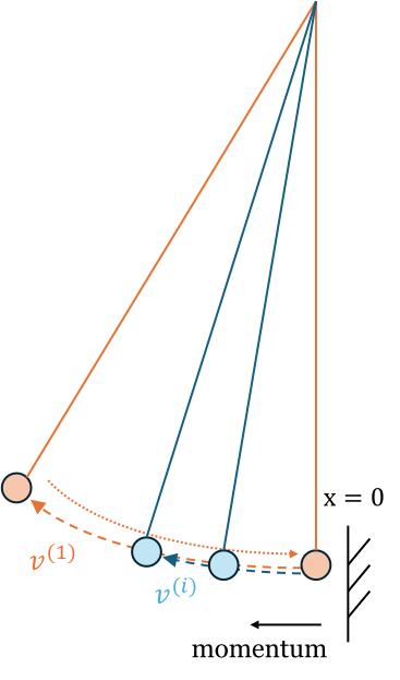
Figure 2 解读：论文用一个理想 wall-bouncing pendulum 解释为什么多尺度 velocity 应该成比例。每次碰墙后，velocity magnitude 按 $α$ 衰减；橙色是 primary trajectory，蓝色是 attenuated trajectories。这个 toy example 不是要精确建模真实摆，而是给 RecFM 一个可训练的结构假设：多条递归轨迹共享方向，但速度幅值按 scale 缩放。

具体地，远离墙面时： $\overset{x}{˙} (t) = v (t), \overset{v}{˙} (t) = 0.$ 碰撞后速度 magnitude 更新为： $v^{(i + 1)} = α v^{(i)},$ 所以经过 $D - 1$ 次碰撞后： $v^{(i)} = α^{(i)} v^{*}, α^{(i)} = α^{i - 1} .$ 这个关系被迁移到 FM：同一个 $x_{t}$ 上的 secondary trajectory target velocity 应是 primary velocity 的缩放版本。若没有这个约束，模型在大步 Euler 推理时只能依赖 primary trajectory 的局部拟合；一旦 learned trajectory 有 curvature 或 scale mismatch，1-step / 2-step 生成会出现明显 truncation error。

3.3 Training objective：trajectory supervision + cross-scale consistency

RecFM 每次训练采样 $x_{0}, x_{1}, t, α$ ，构造共享点 $x_{t}$ ，再对 $D$ 个 scale 做 forward。第 $i$ 条 trajectory 的监督项为： $L_{traj}^{(i)} = \overset{v}{^}^{(i)} - α^{(i)} v^{*}_{2}^{2} .$ cross-scale consistency 项把所有 secondary predictions 对齐到 primary prediction： $L_{cons}^{(i)} = \overset{v}{^}^{(i)} - α^{(i)} \overset{v}{^}^{(1)}_{2}^{2}, i = 2, \dots, D .$ 总目标是： $L_{total} = \sum_{i = 1}^{D} L_{traj}^{(i)} + λ \sum_{i = 2}^{D} L_{cons}^{(i)} .$ 这里 $L_{traj}$ 保证每个 scale 自己有可监督的 target， $L_{cons}$ 保证 scale 之间不会各学各的。论文主实验采用 $D = 2$ 和 $λ = 1$ ： $D = 2$ 已经给出 primary + one secondary trajectory 的核心对齐约束；更大的 $D$ 会引入更多 gradient terms 和显存开销，但收益变小。

3.4 Inference sampling：训练多尺度，推理仍走 primary trajectory

推理时并不需要遍历所有 $α$ 。RecFM 用 learned velocity field 在 $α = 1$ 上解 ODE。1-step Euler 从 noise $x_{1}$ 到 data manifold： $x_{0} \approx x_{1} - h \overset{v}{^}_{θ} (x_{1}, 1, 1), h = 1.$ $K$ -step 推理则按 $1 = t_{0} > \dots > t_{K} = 0$ 更新： $x_{t_{k}} = x_{t_{k - 1}} - h_{k} \overset{v}{^}_{θ} (x_{t_{k - 1}}, t_{k - 1}, 1), h_{k} = t_{k - 1} - t_{k} .$ 训练时的 secondary trajectories 只用于塑造 velocity field；它们不增加推理 NFE。这一点解释了为什么 RecFM 可以在 1-step / 2-step 下比多步 diffusion emulator 快很多：额外成本被放到训练时的多尺度 supervision，而不是推理时的 iterative refinement。

3.5 Theoretical result：通过 trajectory straightening 降低 Euler error

论文把少步生成误差写成 Euler discretization error。若 $h = 1/ K$ ，trajectory acceleration 为： $a (x, t) = \partial_{t} v_{θ} (x, t, 1) + (\nabla_{x} v_{θ}) v_{θ} (x, t, 1),$ 则 $K$ -step Euler error 满足： $ψ_{1} - \hat{ψ}_{1} \leq \frac{h}{2} \frac{e ^{L} - 1}{L} sup_{t \in [0, 1]} ∥ a (ψ_{t}, t) ∥,$ 其中 $L = sup_{t} ∥ \nabla_{x} v_{θ} (\cdot, t, 1) ∥_{op}$ 。Consistency loss 对应的 cross-scale condition 是： $t \partial_{t} v_{θ} (x, t, 1) + v_{θ} (x, t, 1) = \partial_{α} v_{θ} (x, t, 1) .$ 这个条件约束 $\partial_{t} v_{θ}$ ，从而压低 acceleration norm；acceleration 越小，trajectory 越 straight，Euler 大步近似越可靠。换句话说，RecFM 不是让 sampler 更复杂，而是让 learned ODE 更适合大步积分。

3.6 Pseudocode（依据论文 Algorithm 1；released code 尚未发布）

代码搜索未找到开源实现（checked: arXiv/PDF/project links, title+github, acronym+github, arXiv ID, first-author/org candidate repos, GitHub repo/code search; only the official placeholder repo Rose-STL-Lab/RecFM and an empty Hugging Face model page were found）。因此下面伪代码是 paper-grounded pseudocode，不是 released implementation 的逐行转写。

3.6.1 Recursive trajectory training step

import torch
import torch.nn.functional as F
 
 
def recfm_train_step(v_theta, batch, optimizer, lambda_cons: float = 1.0, depth: int = 2):
    x0 = batch["data"]                 # sample from p0
    x1 = torch.randn_like(x0)           # sample from p1
    b = x0.shape[0]
 
    t = torch.rand(b, *([1] * (x0.ndim - 1)), device=x0.device)
    alpha = t + (1.0 - t) * torch.rand_like(t)  # alpha ~ U(t, 1)
 
    v_star = x1 - x0
    x_t = (1.0 - t) * x0 + t * x1
 
    preds = []
    traj_loss = 0.0
    for i in range(depth):
        alpha_i = alpha ** i
        tau_i = t / alpha_i.clamp_min(1e-6)
        v_hat_i = v_theta(x_t, tau_i, alpha_i)
        preds.append((alpha_i, v_hat_i))
        traj_loss = traj_loss + F.mse_loss(v_hat_i, alpha_i * v_star)
 
    cons_loss = 0.0
    primary = preds[0][1]
    for alpha_i, v_hat_i in preds[1:]:
        cons_loss = cons_loss + F.mse_loss(v_hat_i, alpha_i * primary)
 
    loss = traj_loss + lambda_cons * cons_loss
    optimizer.zero_grad(set_to_none=True)
    loss.backward()
    optimizer.step()
    return {"loss": loss.item(), "traj": float(traj_loss), "cons": float(cons_loss)}

3.6.2 One-step and few-step sampling

@torch.no_grad()
def recfm_sample(v_theta, x_noise, num_steps: int = 1):
    x = x_noise
    times = torch.linspace(1.0, 0.0, num_steps + 1, device=x.device)
    for k in range(1, len(times)):
        t_prev = times[k - 1]
        t_next = times[k]
        h = t_prev - t_next
        t_tensor = torch.full((x.shape[0],), float(t_prev), device=x.device)
        alpha_tensor = torch.ones_like(t_tensor)
        v = v_theta(x, t_tensor, alpha_tensor)
        x = x - h * v
    return x

3.6.3 No released implementation mapping

Paper Concept	Source File	Key Class/Function
Recursive trajectory training	N/A	论文 Algorithm 1；released implementation not available
Velocity network $v_{θ} (x, t, α)$	N/A	论文描述基于 HV-DiT backbone；官方 repo 尚无代码
Consistency objective $L_{cons}$	N/A	论文 Eq. (training objective)；无源码可锚定
Forecasting configs / launch scripts	N/A	论文只给 appendix hyperparameter table；无 launch config 可核对

3.7 Architecture and implementation details from paper

论文采用 VideoPDE 的 Hierarchical Video Diffusion Transformer (HV-DiT) backbone，唯一明确修改是移除 input mask channel。这样 RecFM 可以直接作用在 learned velocity field 上，而不是像 DYffusion 那样绑定 forecast-oriented diffusion formulation。由于 released code 未发布，训练配置只能来自 Appendix Table 4，而不是 launch script；论文报告的 Navier-Stokes / $D = 2$ 配置为：116.2M parameters、40k training steps、batch size 64、4×NVIDIA L40S、bfloat16 mixed precision、patch size $[2, 2, 1]$ 、feature dimensions $[384, 768]$ 、AdamW、learning rate $5 \times 1 0^{- 4}$ 、 $[β_{1}, β_{2}] = [0.9, 0.95]$ 、 $λ = 1$ 、weight decay $1 \times 1 0^{- 2}$ 。

论文还指出，递归训练每次 iteration 需要 $D$ 次 forward/backward gradient evaluations；为了让总体训练成本与其他模型可比，作者把训练 iterations 按 $D$ 等比例减少。这一点很重要：RecFM 的推理加速不是免费来自更小模型，而是通过训练时更多 scale supervision 换来推理时更少 NFE。

4. Experimental Setup (实验设置)

4.1 Datasets

Sea Surface Temperatures (SST)：来自 DYffusion benchmark / NOAA OISSTv2，空间分辨率 $1/ 4^{\circ}$ ；使用 eastern tropical Pacific 的 $60 \times 60$ latitude-longitude grid，每个样本包含 11 个 spatial boxes、单通道温度场。论文给出 split：1982–2019 train，2020 validation，2021 test；未给出精确样本条数。
Navier-Stokes Flow：incompressible channel flow past four randomly generated circular obstacles；kinematic viscosity $ν = 1 0^{- 3}$ ，原始 grid 为 $221 \times 42$ ，3 个 channels： $x$ velocity $u$ 、 $y$ velocity $v$ 、pressure $p$ 。RecFM / Vanilla FM / VideoPDE 输入前插值到 $220 \times 40$ ，评估时再 upsample 回 $221 \times 42$ 。论文未给出 train/val/test sample count。
Helmholtz Staircase Equation：来自 The Well，模拟 point source near periodic staircase boundary 的 acoustic scattering；field discretized into $1024 \times 256$ ，2 个主要 channels 为 $R e (U)$ 和 $I m (U)$ ，并把 constant domain masks 作为第三 input channel。论文未给出精确样本条数。
ImageNet-1k image generation appendix：RecFM-XL 在 $256 \times 256$ ImageNet-1k 上评估 FID，使用 CFG=1.5；这是泛化实验，不是主 scientific forecasting benchmark。

4.2 Forecasting protocol

SST 从 1-day input 预测 7 days ahead。Navier-Stokes 从 initial state 进行完整 64-step trajectory reconstruction，autoregressive rollout 中每次生成 16 frames。Helmholtz 从 initial state 重建 49 steps，每次生成 7 frames。概率指标 CRPS / SSR 使用 $M = 50$ ensemble members per initial condition。所有 runtime measurements 在单张 NVIDIA L40S 上测量。

4.3 Baselines and metrics

主 baselines 包括 DYffusion 设置中的 Perturbation、Dropout、DDPM、MCVD、DYffusion；此外加入 VideoPDE 作为 SOTA diffusion/video-inpainting style physics solver，并加入 Vanilla FM（与 RecFM 使用相同 backbone，但没有 recursive training objective）。PBFM 因为需要 closed-form PDE residual，不适用于 SST 这种数据驱动气候场，因此不放入主表，而在 appendix 的 physics-informed evaluation 中比较。Shortcut Model 主要在 Helmholtz 1-step appendix 中比较。

指标包括：CRPS（probabilistic forecast 的 proper scoring rule，越低越好）、MSE（ensemble mean prediction 与 ground truth 的均方误差，越低越好）、SSR（ensemble spread 与 RMSE 的 ratio，越接近 1 越好）。Physics-informed appendix 还报告 Navier-Stokes 的 KE Accuracy（越接近 1 越好）和 Helmholtz 的 PDE Residual（越低越好）。Image generation appendix 报告 FID（越低越好）。

5. Experimental Results (实验结果)

5.1 Main forecasting results

Dataset	Best RecFM	Key numbers	Compared baseline
SST	RecFM 2-step	CRPS 0.216, MSE 0.161, SSR 1.004, Time 0.7353s	与 MCVD 的 CRPS/MSE 持平或略优，但 MCVD time 79.167s；RecFM 1-step time 0.4310s
Navier-Stokes	RecFM 1-step	CRPS 0.031, MSE 0.0064, SSR 0.959	VideoPDE: CRPS 0.033, MSE 0.0068, SSR 0.205；Vanilla FM: MSE 0.0076
Helmholtz	RecFM 2-step / 1-step	2-step: CRPS 0.0027, MSE 2.7e-5；1-step: CRPS 0.0034, MSE 4.2e-5, SSR 1.090	VideoPDE: CRPS 0.026, MSE 5.6e-4, SSR 4.334

论文强调 RecFM 在 Helmholtz 上相对 VideoPDE 有约 $10 \times$ error reduction；相对 diffusion-based emulator VideoPDE 最多有 $20 \times$ speedup；相对 Vanilla FM 的 MSE 降低超过 $15%$ 。优势在 deterministic PDE-governed tasks 上最明显，在 SST 这种更 stochastic 的 real-world climate data 上更接近强 baseline。

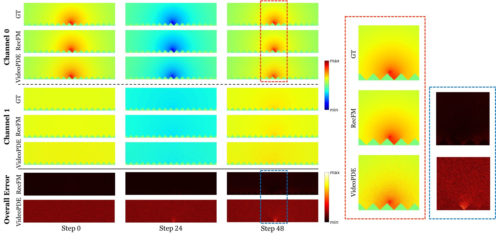
Figure 3 解读：Helmholtz benchmark 中，RecFM 的两个 channels 预测更接近 Ground Truth，bottom rows 的 absolute error 更小；VideoPDE 在圆形波传播结构和 Step 48 的局部变化上误差明显更大。这说明 RecFM 的少步生成并没有牺牲高频/相位结构，反而因为轨迹更 straight，长 rollout 的误差更不容易堆积。

5.2 Training stability and inference-step ablations

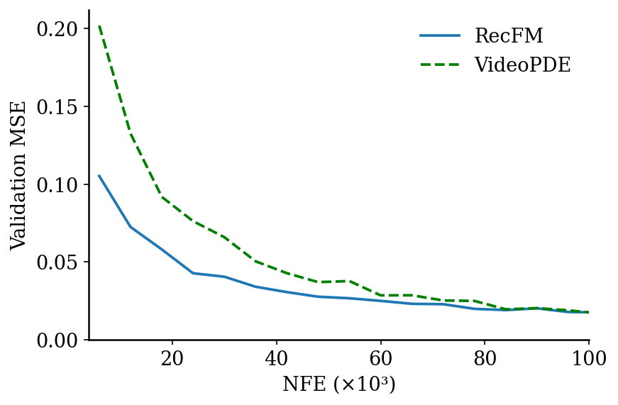
Figure 4 解读：横轴是 training 中累计 function evaluations (NFE)，纵轴是 Navier-Stokes validation MSE。RecFM 比 VideoPDE 更早下降且保持更低误差，说明 recursive trajectory supervision 不只是推理时减少 NFE，也改善了训练过程中的 sample efficiency / convergence stability。

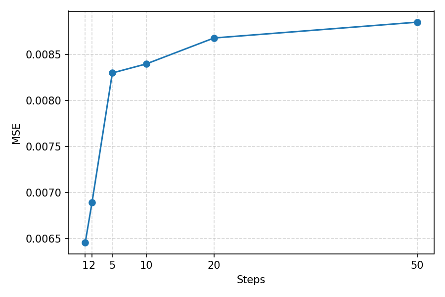
Figure 5 解读：Navier-Stokes 上 RecFM 在 1-step / 2-step 附近达到最佳，继续增加 inference steps 反而可能累积误差。这个现象支持论文的核心设定：RecFM 是为 few-step generation 训练的；在 deterministic physics rollout 中，走更长的 sampling trajectory 未必更好。

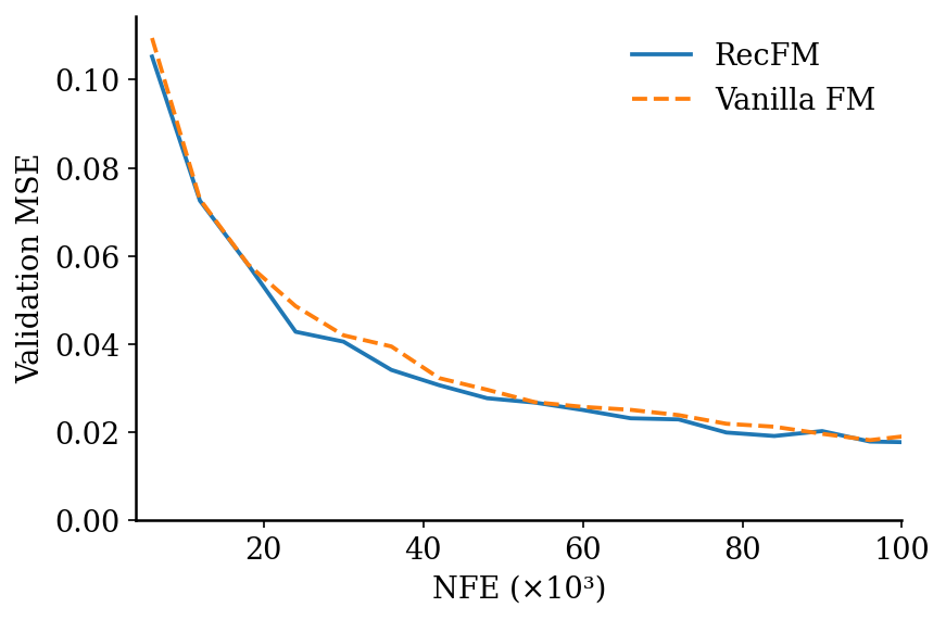
Figure 6 解读：与 Vanilla FM 相比，RecFM 的 validation MSE 更快下降并保持更低。由于两者使用相同 backbone，这个差异主要来自 recursive trajectory loss 和 consistency loss，而不是模型容量差异。

递归深度 ablation 显示：Vanilla FM $D = 1$ 用 5-step inference 时 CRPS 0.036、MSE 0.0076、SSR 0.911、Time 6.914s；RecFM $D = 2$ 用 1-step 时 CRPS 0.031、MSE 0.0064、SSR 0.959、Time 1.588s； $D = 3$ 用 1-step 时 CRPS 0.031、MSE 0.0065、SSR 1.091、Time 1.594s。 $D = 3$ 没有明显提升且需要更多显存，因此主实验采用 $D = 2$ 。

5.3 Consistency weight $λ$ ablation

$λ$	1-step CRPS	1-step MSE	1-step SSR	5-step CRPS	5-step MSE	5-step SSR
0.0	0.035	0.0074	0.957	0.039	0.0093	0.843
0.5	0.034	0.0071	1.024	0.040	0.0099	0.855
1.0	0.031	0.0064	0.959	0.037	0.0083	0.836
10.0	0.038	0.0089	0.988	0.039	0.0089	0.784
$1 0^{6}$	0.238	0.268	1.147	0.234	0.261	1.161

$λ = 1$ 在 CRPS / MSE 上最好，说明 consistency 需要适中权重。 $λ = 0$ 时仍比 Vanilla FM 主表更好，说明 secondary trajectory supervision 本身已有帮助；但 $λ = 1 0^{6}$ 会让 consistency term 压倒 primary FM objective，导致性能崩溃。

5.4 Additional qualitative and physics-informed results

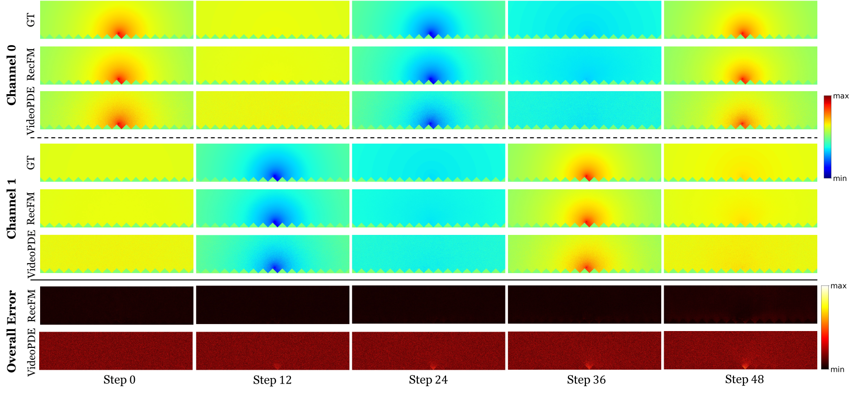
Figure 7 解读：更多 Helmholtz rollout 展示 RecFM 在不同 timestep 和两个 complex channels 上都能保持波场结构。相比之下，baseline 的误差图更集中在波前和边界附近，说明它难以保持 phase-coherent propagation。

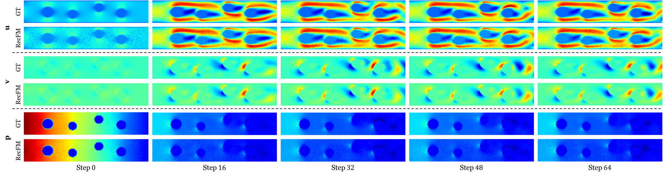
Figure 8 解读：Navier-Stokes rollout 中，RecFM 更好地保持 obstacle 后方复杂涡结构；误差没有沿 autoregressive rollout 快速扩散。这与主表中 RecFM 1-step MSE 0.0064、SSR 0.959 一致，说明少步 velocity field 在流体任务上仍能维持 dynamics。

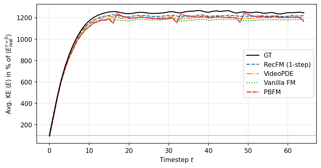
Figure 9 解读：图中是 normalized average kinetic energy $⟨ E (t)⟩ / ⟨ E_{real}^{t = 0} ⟩$ 。RecFM 的曲线更接近 ground truth，Table 6 中 Navier-Stokes KE Accuracy 达到 0.9791（1-step），优于 VideoPDE 0.9670、Vanilla FM 0.9522 和 PBFM 0.9592；这说明 RecFM 不是只优化 pixel MSE，也更好保留物理能量演化。

Physics-informed appendix 进一步显示：在 Navier-Stokes 上 RecFM 1-step 的 CRPS/MSE/SSR/KE Accuracy/Time 为 0.031 / 0.0064 / 0.959 / 0.9791 / 1.588s；PBFM 为 0.034 / 0.0071 / 0.810 / 0.9592 / 14.75s。在 Helmholtz 上 RecFM 2-step 的 PDE Residual 为 0.00457，低于 RecFM 1-step 0.00476、PBFM 0.00519、VideoPDE 0.00841 和 Vanilla FM 0.01102。

Shortcut comparison（Helmholtz 1-step）显示 Shortcut Model CRPS 0.0144、MSE 1.6e-4、SSR 0.467，而 RecFM 为 CRPS 0.0034、MSE 4.2e-5、SSR 1.090；这说明 RecFM 的 velocity-scale consistency 比直接 shortcut-style one-step baseline 更适合这个 PDE rollout。

5.5 Image generation appendix

Model	FID ↓	Sampling Steps	Param Count	Epochs Trained
DiT-XL	2.27	500	675M	640
SiT-XL	2.06	250	675M	640
ADM-G	4.59	250	—	426
LDM-4-G	3.6	500	400M	106
Shortcut Model (XL)	3.8	128	676M	250
RecFM-XL	2.53	128	675M	160
RecFM-XL	2.49	16	675M	160
RecFM-XL	3.22	8	675M	160

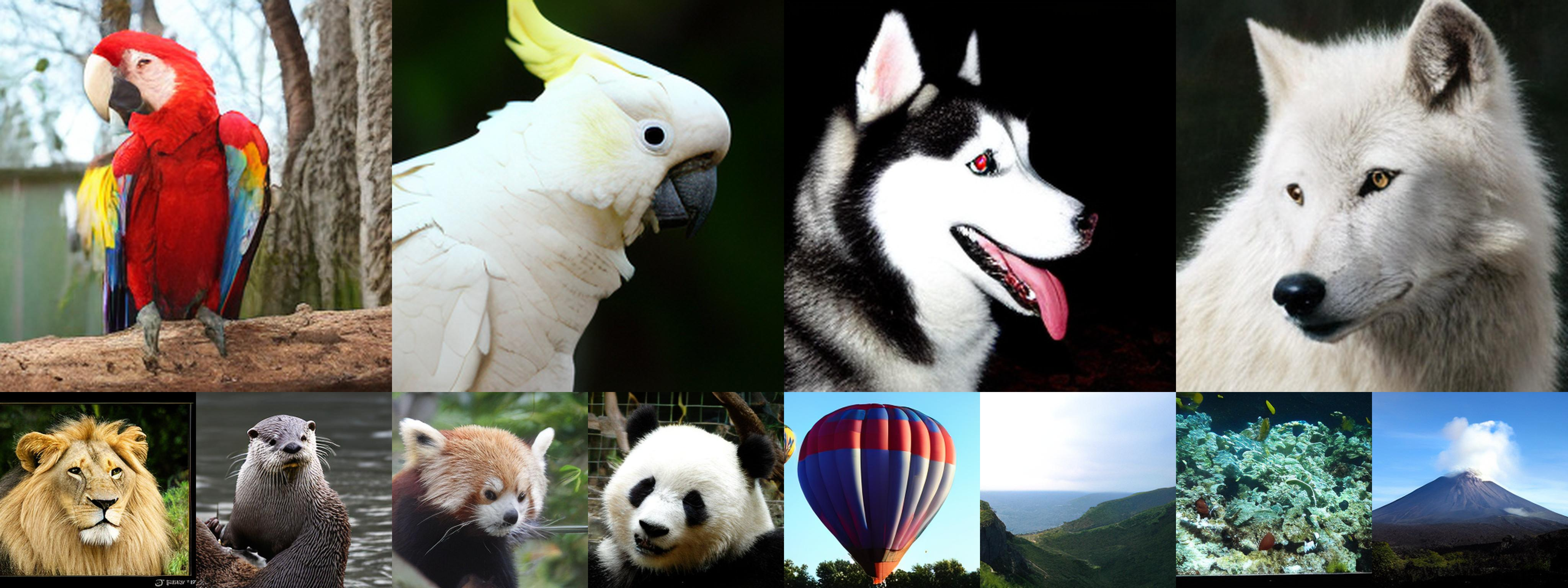
Figure 10 解读：RecFM-XL 在 ImageNet-1k 上能生成 $256 \times 256$ 样本，并在 16 steps 达到 FID 2.49。值得注意的是，128 steps 的 FID 2.53 反而略差于 16 steps，符合论文对 few-step objective 的解释：RecFM 的训练目标强化少步生成，因此更多 sampling steps 不一定继续改善质量。

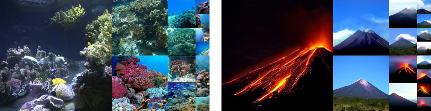
Figure 11 解读：这是 uncurated ImageNet 类别样本的第一组（Coral reef / Volcano）。它们不是主 scientific benchmark 的证据，而是说明 RecFM 的递归轨迹思想可以从物理场扩展到通用图像生成。

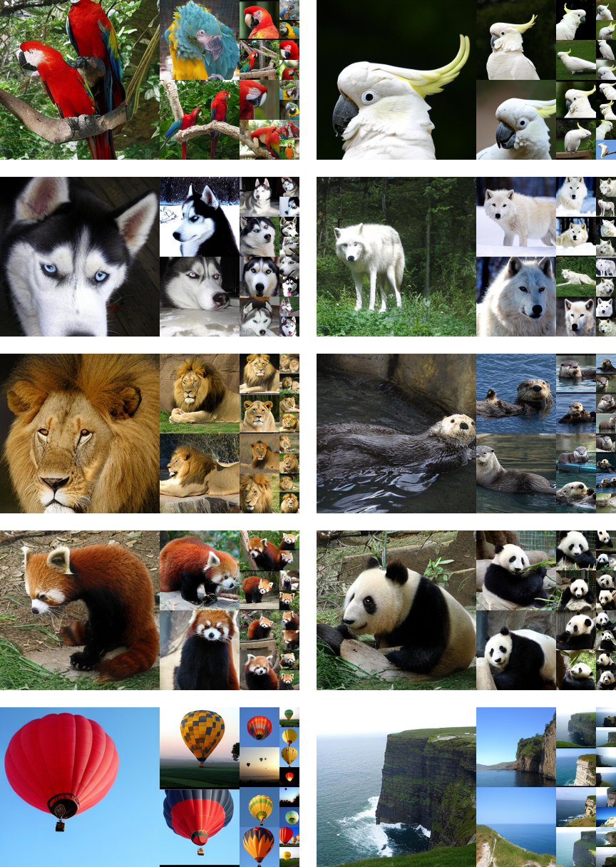
Figure 12 解读：继续展示 Macaw、Cockatoo、Husky、Arctic wolf、Lion、Otter、Red panda、Panda、Balloon、Cliff drop-off 等类别。图像 appendix 的主要结论不是 RecFM 超越 DiT/SiT 的最终质量，而是用更少训练 epochs 和更少 inference steps 达到有竞争力的 FID。

5.6 Limitations and takeaways

作者明确讨论的 caveat 是：RecFM 对 deterministic / PDE-governed tasks 的优势更强，对 SST 这种 stochastic real-world climate field 的提升较小；多步 RecFM 不总是优于单步，因为后续 step 也会累积误差；此外 released implementation 尚未发布，训练细节只能从论文 appendix table 复核，不能检查 actual launch script / config。总体结论是：RecFM 把 cross-scale velocity alignment 注入 Flow Matching，使 learned trajectory 更适合大步 Euler integration，在 scientific emulation 中用 1–2 steps 获得接近或超过多步 diffusion emulator 的 accuracy、calibration 和 physics consistency。

Paper Notes

探索

Recursive Flow Matching

Recursive Flow Matching

1. Motivation (研究动机)

2. Idea (核心思想)

3. Method (方法)

3.1 Overall framework：从单条 FM 轨迹扩展到递归多尺度轨迹

3.2 Physics intuition：wall-bouncing pendulum 的速度缩放

3.3 Training objective：trajectory supervision + cross-scale consistency

3.4 Inference sampling：训练多尺度，推理仍走 primary trajectory

3.5 Theoretical result：通过 trajectory straightening 降低 Euler error