Image-Free Timestep Distillation via Continuous-Time Consistency with Trajectory-Sampled Pairs

Paper: arXiv:2511.20410 Code: hustvl/TBCM Code reference: main @ c6a45836 (2025-12-16)

1. Motivation (研究动机)

这篇论文要解决的是 text-to-image diffusion model 的一步或少步生成加速问题，但它的切入点不是再设计一个更强的采样器，而是重新审视 timestep distillation 里“训练样本从哪里来”。扩散模型在图像与视频生成中质量很强，但标准推理通常需要几十甚至上百步 denoising；即使底层模型只有 0.6B 参数，反复调用 teacher 或 student 仍会让 latency 和显存成为部署瓶颈。timestep distillation 的目标是把多步生成过程压缩到一个 student，让 student 在 1-step 或 few-step 下直接给出高质量样本。Consistency Model (CM) 和 Continuous-Time Consistency Distillation (CTCD) 的吸引力在于：它们不必像早期 progressive distillation 那样显式保存大量 teacher samples，也不必像 adversarial distillation 那样引入额外判别器不稳定性，而是要求同一条 probability flow ODE 上不同噪声水平的预测保持一致。

问题在于，现有连续时间 consistency distillation 仍沿用“真实图像或预生成图像 → VAE 编码 → 加噪得到 $x_{t}$ ”的范式。对于 latent diffusion / flow matching 系统，这带来两个直接成本。第一，VAE 编码和图像数据管线占据大量显存，尤其当 batch size 增大时，VAE encode 阶段会成为最显著的动态显存峰值。第二，text encoder 的 prompt encoding 虽然不一定是显存最大项，但在训练时间里占据相当比例；如果每个 prompt 只产生一个训练点，text embedding 的开销无法摊薄。论文在 Figure 4 中把这两个瓶颈拆开：显存分解显示 VAE encoding 约占动态显存消耗的 80%；时间分解显示 Data Loader 和 VAE Encoding 不到 1%，Text Encoder 与 Diffusion Distillation 本身同量级，因此“图像数据 + 单点采样”的流程既重又不够高效。

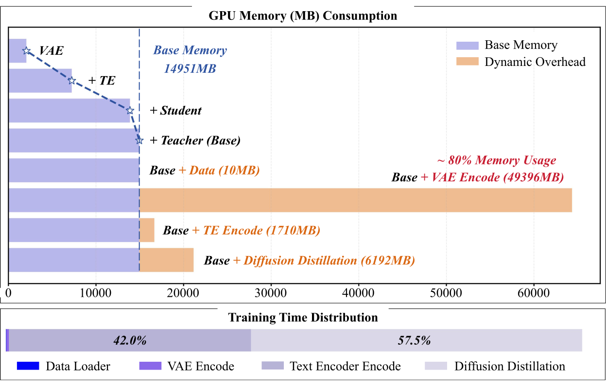
Figure 1 解读：上半部分说明显存瓶颈主要来自 VAE Encode 这个阶段，而不是固定加载的 teacher/student/text encoder；下半部分说明训练耗时并不是 data loader 本身，而是 prompt encoding 与 diffusion distillation 的组合。这个观察直接支持 TBCM 的两个设计：不再需要真实图像的 VAE 编码，并且一个 prompt 沿 teacher trajectory 生成多个训练点来摊薄 text encoder 开销。

更深层的问题是 training–inference inconsistency。传统 sCM / Sana-Sprint 在训练时构造的是 diffusion space 样本：固定某个 clean image $x_{0}$ ，再对它添加不同强度的噪声得到 $(x_{t}, t)$ 。但模型推理时实际走的是从纯噪声出发的 backward generation trajectory；这条轨迹上的 $x_{t}$ 并不是“同一个真实图像加噪”的结果，而是 teacher 在逐步去噪过程中形成的中间状态。论文用 Equivalent Noise $N o i s e_{e q v} = \frac{x _{t} - c o s ( t ) x ^ _{0}}{s i n ( t )}$ 刻画这种差异：在 forward diffusion 中，等价噪声应基本保持一致；在 backward generation 中，它会逐步从随机噪声演化成与预测目标相关的结构性模式。这说明传统 CTCD 约束的样本空间与实际推理路径不对齐，student 学到的一致性约束可能正好施加在“推理时很少遇到”的区域。

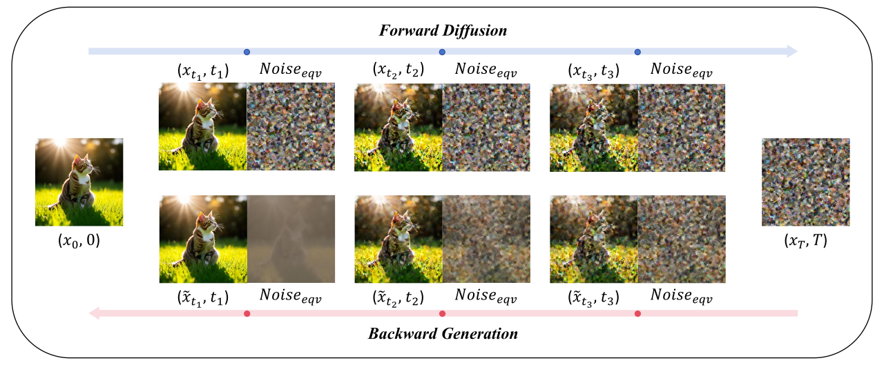
Figure 2 解读：该图比较 forward process 和 backward process 中 equivalent noise 的演化。Forward 里噪声近似不变，符合“固定 $x_{0}$ 加噪”的训练假设；Backward 里噪声分布随时间明显变化，说明推理轨迹包含 teacher 逐步形成语义与结构的过程。TBCM 的 motivation 正是把 distillation sample 从 forward diffusion space 移到 generation space。

因此，这篇论文的核心问题可以概括为：能否不依赖任何外部图像数据，直接从 teacher 的生成轨迹中抽取 $(x_{t}, t)$ 样本对来训练 continuous-time consistency student？如果可以，收益不仅是省掉数据与 VAE 编码，更是把训练约束放到模型真正推理时经过的区域。这个问题值得研究，因为它把 timestep distillation 从“需要高质量 image dataset 的压缩流程”变成“只需要 prompt 与 teacher 的自包含蒸馏流程”，对资源受限场景、跨领域迁移、以及未来 text-to-video / audio-video diffusion 加速都有现实意义。

2. Idea (核心思想)

TBCM 的核心 insight 是：continuous-time consistency distillation 的训练样本不必来自真实图像加噪；更自然的样本源是 teacher model 自己的 backward generation trajectory。给定 prompt 和初始噪声，teacher 在 TrigFlow / flow matching 路径上产生一串中间 latent；TBCM 直接收集这些 latent states 与对应的时间点，把它们作为 consistency loss 的训练输入。这样一来，student 学到的是 teacher 实际推理路径上的局部一致性，而不是 forward diffusion 人工构造出来的样本空间。

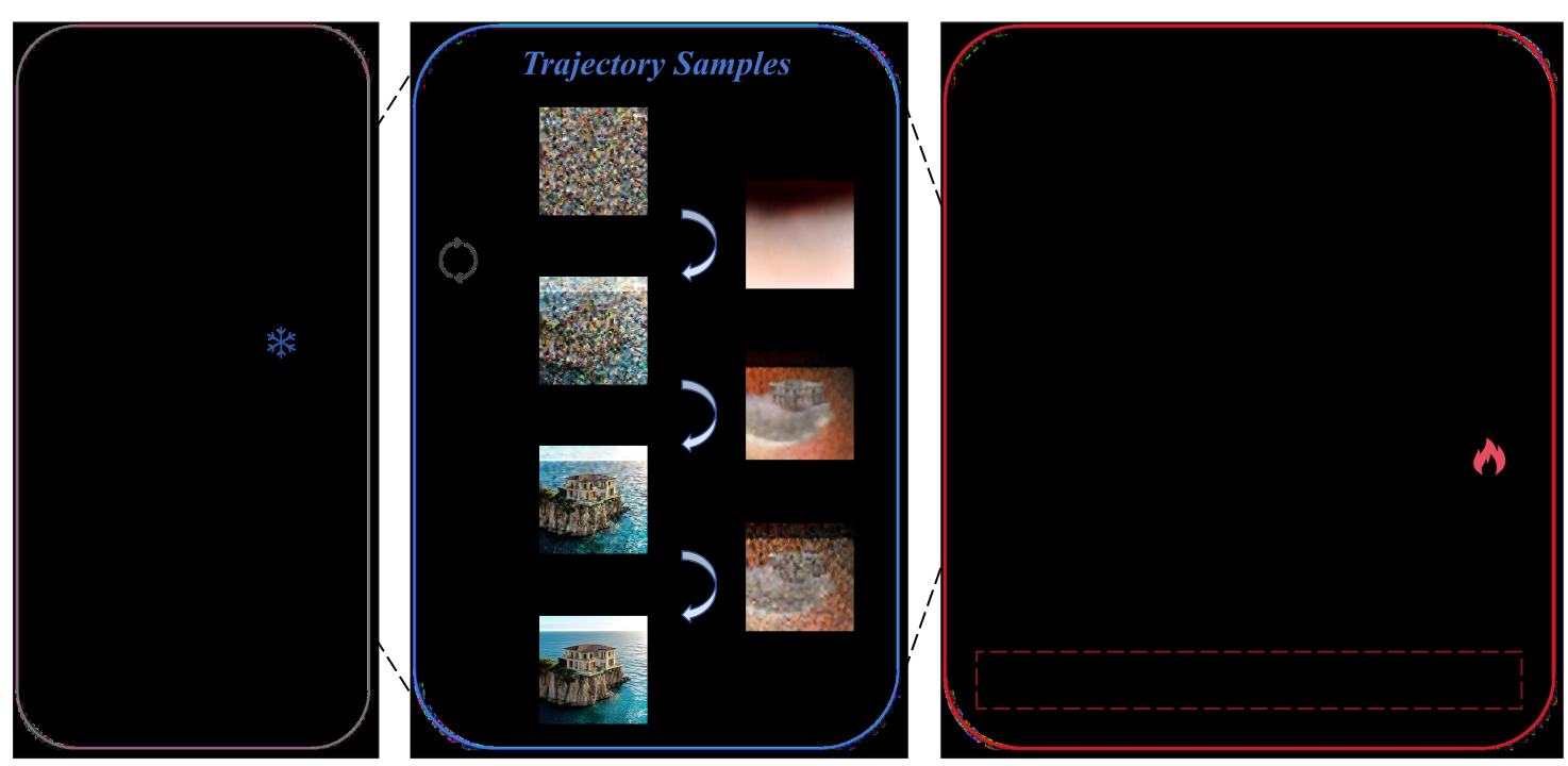
Figure 3 解读：左侧从随机噪声和文本 prompt 开始，中间由 teacher 在 latent space 内生成多步 trajectory samples，右侧把这些 samples 送入 continuous-time consistency loss。关键变化是“图像样本 → VAE 编码 → 加噪”的流程被替换为“prompt → teacher trajectory → latent pair”，所以它同时解决了 image-free、显存、训练时间、训练/推理空间对齐四个问题。

与 Sana-Sprint / sCM 相比，TBCM 不是只改 loss 的某个权重，而是换掉 distillation sample 的来源。Sana-Sprint 仍然在 diffusion space 里按 logit-normal timestep 采样；TBCM 则在 generation space 中采样，样本不仅受时间点 $t$ 控制，也受整条 denoise route 的历史影响。论文进一步提出 Reference Route：先用 Flow-Euler Scheduler 的带 shift 时间表得到一条参考轨迹，再在各个区间内采样，使每条 trajectory 覆盖多个子区域，而不是随机丢点。这是它与“直接随机采样 timestep”的根本差别。

TBCM 还包含两个实用补丁。第一是 Brightness Filter：teacher 轨迹末端可能产生低质量、异常偏暗的 $\overset{x}{^}_{0}$ ；为了保持 image-free，它不解码到像素空间判断，而是预先保存全黑图像的 latent，用 latent-space MSE 筛掉过近的样本。第二是 stability hyperparameter $R$ ：sCM 中对不稳定项的 $sin (t)$ warmup 最终值不一定应为 1.0，TBCM 实验发现 $R_{f ina l} = 0.75$ 与 Warmup–Cooldown schedule 更稳。直观上，TBCM 把“样本从哪里来”和“loss 中不稳定切向项怎么加权”一起调到更适合 generation-space distillation 的状态。

3. Method (方法)

3.1 预备公式：从 diffusion / flow 到 TrigFlow consistency

论文采用 TrigFlow 记号来承接 Sana-Sprint 与 sCM。一般扩散扰动可写为 $x_{t} = α_{t} x_{0} + σ_{t} z, z \sim N (0, I) .$ 在 TrigFlow 中， $α_{t} = cos t$ ， $σ_{t} = sin t$ ， $t \in [0, π /2]$ ，sampling ODE 由 $\frac{d x _{t}}{d t} = σ_{d} F_{θ} (\frac{x _{t}}{σ _{d}}, t)$ 表示。Consistency Model 学一个函数 $f_{θ} (x_{t}, t)$ ，要求沿 ODE 轨迹不同时间点的 clean prediction 保持一致。离散 CM 用相邻时间点 loss： $l_{CM}^{Δ t} = E_{x_{t}, t} [d (f_{θ} (x_{t}, t), f_{θ^{-}} (x_{t - Δ t}, t - Δ t))],$ 连续时间版本取 $Δ t \to 0$ ，得到 $l_{CM}^{co n t .} = E_{x_{t}, t} [w (t) ⟨ f_{θ} (x_{t}, t), \frac{d f _{θ^{-}}}{d t} (x_{t}, t) ⟩] .$ 难点在于 $\frac{d f _{θ^{-}}}{d t}$ 的稳定计算。sCM / Sana-Sprint 在 TrigFlow 下把它改写成含有 model output、 $x_{t}$ 、以及 $d F_{θ^{-}} / d t$ 的表达式，并通过 JVP 与 tangent normalization 稳定训练。TBCM 沿用这个 continuous-time objective，但换掉 $x_{t}$ 的来源：不是从 VAE-encoded image 加噪，而是沿 teacher generation trajectory 采样。

3.2 Trajectory-Backward Consistency：从 teacher ODE 收集训练对

TBCM 从 prompt $y$ 和初始噪声 $x_{π /2} \sim N (0, σ_{d}^{2} I)$ 出发，显式模拟 teacher 的 denoising trajectory： $\frac{d x _{t}}{d t} x_{t - Δ t} = F_{t e a c h er} (\frac{x _{t}}{σ _{d}}, t), = cos (Δ t) x_{t} - sin (Δ t) σ_{d} \frac{d x _{t}}{d t} .$ 实际代码中 train_scripts/train_tbcm.py 对每个 batch 先采样 x_t = torch.randn(...) * sigma_data，再调用 pretrained_model(x_t / sigma_data, t, **model_kwargs) 得到 teacher prediction，并令 dxt_dt = sigma_data * pretrain_pred。每走一步都把当前 latent state 放入 all_preds，把 teacher derivative 放入 all_dxt_dt，最后把除了第一个初始点外的 trajectory states 拼接成训练样本。这样，一个 prompt 不只产生一个 $(x_{t}, t)$ ，而是产生一串 time-ordered samples；这些样本共享同一个文本 embedding，因此 text encoder 成本被摊薄。

def collect_teacher_trajectory(pretrained_model, prompt_embed, route, sigma_data, cfg_scale=None):
    x_t = torch.randn(batch, latent_dim, h, w, device=device) * sigma_data
    states, derivatives, times = [], [], []
    with torch.no_grad():
        for i, t_i in enumerate(route):
            states.append(x_t.detach())
            t = torch.full((batch, 1, 1, 1), t_i, device=device)
            times.append(t)
            pred = pretrained_model(x_t / sigma_data, t.flatten(), y=prompt_embed.y, mask=prompt_embed.mask)
            dxt_dt = sigma_data * pred
            derivatives.append(dxt_dt.detach())
            dt = route[i] if i == len(route) - 1 else route[i] - route[i + 1]
            x_t = torch.cos(dt) * x_t - torch.sin(dt) * dxt_dt
    return torch.cat(states[1:]), torch.cat(derivatives[1:]), torch.cat(times[1:]), x_t

这段伪代码对应 released code 的核心训练路径。注意它不是“先生成图像再 VAE encode”，也不是使用真实 image dataset；数据集只需 prompt 文本文件，配置中 data.data_dir: [./prepare/data/prompts.txt]，data.type: SanaTextDataset，data.load_vae_feat: false。这解释了论文为什么称其为 image-free：VAE 只在 validation 可视化时 decode latent，不参与训练样本构造。

3.3 Sampling scheme：generation space 中不仅要采样 timestep，还要采样 route

在 diffusion space 中，clean image 固定，采样策略主要决定噪声强度分布；在 generation space 中， $x_{t}$ 还取决于之前经过的所有中间时间点。因此 TBCM 的采样问题是 trajectory-level 的。论文比较三种策略：Random 在 $[0, π /2]$ 均匀采 $N$ 个点；Logit-Normal 复用 Sana-Sprint 的 $P_{m e an} = 0.2$ 、 $P_{s t d} = 1.6$ ；Reference Route 先通过 Flow-Euler Scheduler 和 schedule shift 构造参考时间表，再把区间分块采样，保证一条轨迹覆盖多个子区域。

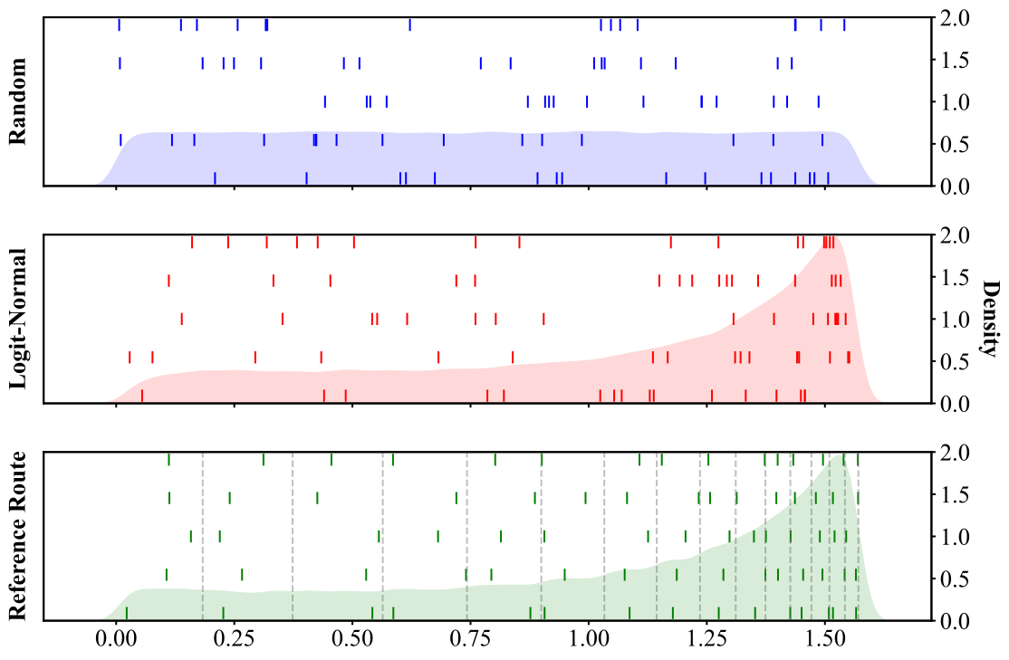
Figure 4 解读：从上到下分别是 Random、Logit-Normal、Reference Route；竖线表示若干随机实例，阴影表示采样密度。Logit-Normal 与 Reference Route 在整体密度上相近，但 Reference Route 额外约束每条 route 在多个区间都有样本，降低了 trajectory 内部 coverage 的随机性，这也是它在 ablation 中优于 Logit-Normal 的原因。

released code 中 diffusion/utils/tbcm_utils.py 的实现分两步：compute_refer_route 先构造带 shift 的 Flow-Euler 风格 reference route，然后用 $arctan (\frac{t}{1000 - t})$ 映射到 TrigFlow 时间；sample_ordered_timesteps_from_ref 在相邻 reference points 之间均匀采一个点，并保持降序。训练脚本调用 compute_refer_route(shift=2.5, num_inference_steps=config.scheduler.route_steps)，而 configs/600M_1024px_tbcm.yaml 把 route_steps 设为 16。

def sample_reference_route(num_train_timesteps=1000, route_steps=16, shift=2.5):
    timesteps = torch.linspace(1000, 1, 1000)
    sigmas = timesteps / num_train_timesteps
    sigmas = shift * sigmas / (1 + (shift - 1) * sigmas)
    # pick route_steps reference points, convert FM-style sigma to TrigFlow t
    ref = torch.atan((sigmas_to_timesteps[1:]) / (1000 - sigmas_to_timesteps[1:]))
    ref = torch.cat([torch.tensor([1.5708], device=ref.device), ref])
    samples = [ref[0:1]]
    for high, low in zip(ref[:-1], ref[1:]):
        samples.append(torch.empty(1, device=ref.device).uniform_(low.item(), high.item()))
    return torch.cat(samples)

3.4 Brightness Filter：不解码图像也能过滤暗样本

teacher trajectory 的末端 $x_{0}$ 有时质量较差，论文观察到这些低质量样本常表现为异常偏暗。为了不破坏 image-free 设定，TBCM 不把 latent decode 成 pixel image 后再计算亮度，而是提前计算全黑图像的 latent 表示 black_latent.pt，训练时对最终 $x_{0} / σ_{d a t a}$ 与 black latent 计算 MSE；过近的样本被 mask 掉。论文附录 Figure “Brightness Filter” 说明了这个策略。

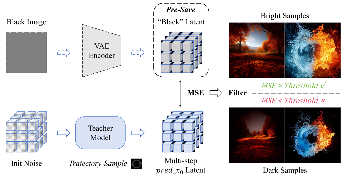
Figure 5 解读：该图把异常暗样本与全黑 latent 的相似性作为过滤依据。它不是一个需要训练的额外 quality model，也不需要 VAE decode；因此它与 TBCM 的低成本设定一致。代价是这个过滤器只能覆盖“过暗”这一类明显失败，不能识别所有 teacher bias 或语义错误。

def brightness_filter(x0_latent, black_latent, threshold=1.0):
    # mirrors diffusion/utils/tbcm_utils.py::black_filter
    mask = torch.ones(x0_latent.shape[0], device=x0_latent.device)
    for i in range(x0_latent.shape[0]):
        mse = F.mse_loss(x0_latent[i], black_latent[i], reduction="mean").item()
        if mse < threshold:
            prob = 1 - mse / threshold
            if random.random() < prob:
                mask[i] = 0.0
    return mask

论文公式与 released code 实现差异：论文只把 Brightness Filter 描述为 latent-space threshold filtering；released code 进一步用 prob = 1 - mse / threshold 做概率式丢弃，而不是小于阈值就确定性过滤。另外，diffusion/utils/tbcm_utils.py 中 black_filter 使用 random.random() 但该文件没有显式 import random；换句话说，random.random() 但该文件没有显式导入 random。如果执行到该分支，当前 release 需要补上 import 或改成 torch.rand 才完全稳健。这不改变论文方法本身，但复现实验时必须检查。

3.5 Continuous-time consistency loss 与 $R$ 调整

TBCM 保留 sCM 的 JVP-based continuous-time consistency loss。训练时先对 student 调一次 torch.func.jvp，得到 $F_{θ}$ 对 $(x_{t}, t)$ 的切向导数；然后构造目标切向量 $g$ ： $g = - cos^{2} (t) (σ_{d} F_{θ^{-}} - \frac{d x _{t}}{d t}) - r \cdot (cos (t) sin (t) x_{t} + σ_{d} \frac{d F _{θ^{-}}}{d t}) .$ 代码中还做 tangent normalization： $g \leftarrow \frac{g}{∥ g ∥ + 0.1} .$ 最终 loss 是带 adaptive log-variance 的平方误差： $L = \frac{w ( t )}{e x p ( l o g σ ^{2} )} ∥ F_{θ} - F_{θ^{-}} - g ∥_{2}^{2} + lo g σ^{2},$ 并乘上 Brightness Filter 的 mask。released config 中 scm_lambda=1.0 来自 diffusion/utils/config.py 默认值，训练脚本用 total_loss = config.train.scm_lambda * loss。

def tbcm_consistency_loss(model, x_t, t, dxt_dt, y, mask, black_mask, sigma_data, global_step, cfg):
    def model_wrapper(scaled_x_t, t_in):
        return model(scaled_x_t, t_in.flatten(), y=y, mask=mask, return_logvar=True, jvp=True)
 
    with torch.no_grad():
        F_theta_minus, F_theta_grad, logvar = torch.func.jvp(
            model_wrapper,
            (x_t / sigma_data, t),
            (torch.cos(t) * torch.sin(t) * dxt_dt / sigma_data, torch.cos(t) * torch.sin(t)),
            has_aux=True,
        )
    F_theta, logvar = model(x_t / sigma_data, t.flatten(), y=y, mask=mask, return_logvar=True, jvp=False)
 
    r = min(1.0, global_step / cfg.train.tangent_warmup_steps)
    progress = (global_step - cfg.train.start_calmdown_step) / cfg.train.tangent_calmdown_steps
    progress = min(max(progress, 0.0), 1.0)
    r = r * (1 - progress) + cfg.train.final_r * progress
 
    g = -torch.cos(t) ** 2 * (sigma_data * F_theta_minus.detach() - dxt_dt)
    g += -r * (torch.cos(t) * torch.sin(t) * x_t + sigma_data * F_theta_grad.detach())
    g = g / (torch.linalg.vector_norm(g, dim=(1, 2, 3), keepdim=True) + 0.1)
    l2 = torch.square(F_theta - F_theta_minus.detach() - g)
    loss = ((1 / (torch.tan(t) * sigma_data)) / torch.exp(logvar.view(-1, 1, 1, 1))) * l2 + logvar.view(-1, 1, 1, 1)
    return (loss * black_mask.view(-1, 1, 1, 1)).mean()

3.6 Source-code mapping

Code reference: main @ c6a45836 (2025-12-16) — pseudocode and mapping based on this commit

Paper Concept	Source File	Key Class/Function
TBCM training loop / teacher trajectory sampling	`train_scripts/train_tbcm.py`	`train`, loop around `compute_refer_route`, `pretrained_model`, `all_preds`, `all_dxt_dt`
Reference Route / ordered trajectory timesteps	`diffusion/utils/tbcm_utils.py`	`compute_refer_route`, `sample_ordered_timesteps_from_ref`
Brightness Filter	`diffusion/utils/tbcm_utils.py`; `train_scripts/train_tbcm.py`	`black_filter`; use of `black_latent.pt` and `black_mask_expand`
Continuous-time sCM/TBCM loss	`train_scripts/train_tbcm.py`	`torch.func.jvp`, construction of `g`, logvar-weighted loss
TrigFlow ↔ Flow output transform	`diffusion/model/nets/sana_multi_scale.py`	`SanaMSCM.forward`
Released training config	`configs/600M_1024px_tbcm.yaml`; `train_scripts/train_tbcm.sh`	1024px SanaMSCM 0.6B, `route_steps=16`, `lr=1e-5`, 4 nodes × 8 GPUs launch defaults

released code 与 paper 的关系需要小心读：论文表格报告的是实验设置与结果，released YAML 是公开复现 recipe。比如论文主表的 training cost 写的是 512 * 20000 total training samples，而 YAML 中 train_batch_size=1 是进程级配置，launch script 默认 np=8、nodes=4，实际全局 batch 还取决于分布式、数据采样和可能的命令行覆盖。再如论文 ablation 显示 sampling steps=20 时 FID 最优，但公开 YAML 默认 route_steps=16；因此不能把 YAML 默认值机械等同于论文每一行表格的最终实验设置。

4. Experimental Setup (实验设置)

数据方面，TBCM 不使用 paired image data。论文写明训练时直接收集 1M 随机文本 prompts；released README 也要求用户准备一个文本文件，每行一个 prompt。评测数据集是 MJHQ-30k，用于 text-to-image 质量评估。评测指标有两个：FID $↓$ 衡量生成分布与参考图像分布的距离，越低越好；CLIP Score $↑$ 衡量图文对齐，越高越好。论文主实验聚焦 one-step generation，并补充了 2-step、4-step generation 的可视化。

Figure 6 解读：这是论文展示的 1024×1024 one-step generation 结果，用来说明 TBCM 在只调用一步 student 的情况下仍能保持较细致的结构和纹理。它不是定量证据本身，但与主表的 FID/CLIP 共同说明：TBCM 的效率提升没有以明显视觉崩坏为代价。

模型与硬件设置如下。teacher 是官方 Sana-Sprint 0.6B teacher model；论文所有训练时间测量在 4 nodes、共 32 张 NVIDIA V100 32GB 上进行，显存测量在单张 A100、batch size 16 下进行。released config configs/600M_1024px_tbcm.yaml 对应 SanaMSCM_600M_P1_D28，image_size=1024，mixed_precision=bf16，cfg_embed=true，teacher 与初始化权重均指向 ./prepare/model/Sana_Sprint_0.6B_1024px_teacher.pth；VAE 配置是 AutoencoderDC，vae_latent_dim=32，vae_downsample_rate=32，但训练数据配置 load_vae_feat=false，符合 image-free latent trajectory 的叙述。

训练超参数中，released YAML 指定 route_steps=16、logit_mean=0.2、logit_std=1.6、sigma_data=0.5、train_batch_size=1、num_epochs=100、gradient_accumulation_steps=1、grad_checkpointing=true、optimizer 为 CAMEWrapper、学习率 1.0e-5、num_warmup_steps=5000、tangent_warmup_steps=4000、scm_cfg_scale=[4,4.5,5]。final_r=0.75、start_calmdown_step=15000、tangent_calmdown_steps=2000 和 scm_lambda=1.0 没有在 TBCM YAML 中覆盖，而是来自 diffusion/utils/config.py 的默认值；这类数字在笔记中应按代码来源标注，不能误称为 YAML override。

比较方法包括预训练模型 SDXL、PixArt- $Σ$ 、SANA，以及蒸馏方法 SDXL-LCM、PixArt-LCM、PixArt-DMD、PCM、SDXL-DMD2、Sana-Sprint、sCM 和 TBCM。主表中的 baseline 结果主要来自 Sana-Sprint report。实验设置的公平性来自两个方面：TBCM 使用同一个 Sana-Sprint 0.6B teacher，并且除 trajectory sampling 带来的轻微 learning-rate 调整外尽量遵循 Sana-Sprint 训练配置；但由于它的数据来源改为 prompt-only + teacher trajectory，实际训练成本结构与 Sana-Sprint/sCM 不同。

附录还做了 generation-space 分布验证与采样策略可视化。Equivalent noise 的 t-SNE 结果显示，forward diffusion 的 equivalent noise 分布保持较稳定，而 generation process 的分布会逐步偏离初始噪声；这为“forward samples 与 backward trajectory 不同分布”提供了分布级证据，而不仅是单个样本的可视化现象。

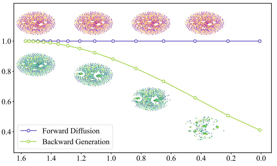
Figure 7 解读：曲线部分展示不同时间点 equivalent noise 与初始噪声的 cosine similarity，散点部分展示 t-SNE 分布。Forward diffusion 近似保持噪声分布，backward generation 则出现明显 pattern change。这支撑了 TBCM 的关键实验假设：generation-space samples 更贴近 student 真正要学习的一步生成路径。

5. Experimental Results (实验结果)

主结果显示，TBCM 在 MJHQ-30k one-step generation 中取得 FID 6.52、CLIP 28.08。与 Sana-Sprint 的 FID 7.04、CLIP 28.04 相比，TBCM 在相同 0.6B 参数、相同 throughput 7.22 samples/s、相同 latency 0.21s 的设置下提升了 FID，并略微提升 CLIP。与 sCM 的 FID 7.46、CLIP 27.74 相比，提升更明显。和预训练 SANA 的 FID 5.81、CLIP 28.36 相比，TBCM 仍有质量差距，但它只需要 1 inference step，而 SANA 表中是 20 steps；所以主结论不是“超过完整多步 teacher”，而是“在一步蒸馏设置下比同类蒸馏方法更接近 teacher”。

Method	Steps	Throughput	Latency	Params	FID ↓	CLIP ↑
SANA	20	1.7	0.9	0.6B	5.81	28.36
SDXL-DMD2	1	3.36	0.32	2.6B	7.10	28.93
Sana-Sprint	1	7.22	0.21	0.6B	7.04	28.04
sCM	1	7.22	0.21	0.6B	7.46	27.74
TBCM	1	7.22	0.21	0.6B	6.52	28.08

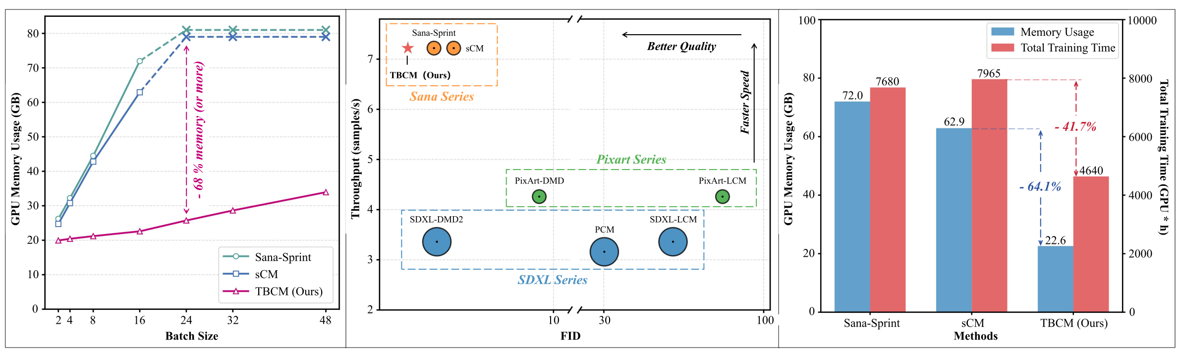
Figure 8 解读：左图对比训练显存随 batch size 的变化，中图把 FID、throughput 和参数量放到同一张图上，右图对比显存与总训练时间。它把 TBCM 的优势显示成一个 Pareto trade-off：不是牺牲速度换质量，也不是单纯减少参数，而是在相同 0.6B student 和相同推理速度下，通过换 sample source 降低训练成本并改善一步质量。

训练成本表更能体现 image-free 的收益。Sana-Sprint 的 average sample time 是 2.7 GPUs，显存 72.0GB，总训练时间 7680 GPUh；sCM 是 2.8 GPUs，62.9GB，7965 GPUh；TBCM 是 1.6 GPUs，22.6GB，4640 GPUh。相对于 sCM，TBCM 显存降低 64.1%，总训练时间降低 41.7%；相对于 Sana-Sprint，也大幅减少显存并减少约 40% 训练时间。这里的关键不是 VAE encode 时间本身很长，而是移除 VAE 和图像数据后，每个 prompt 可产生多个 trajectory samples，从而让整体 sample efficiency 与显存峰值都改善。

定性比较也支持这个结论。论文 Figure 6（此处按笔记编号 Figure 9）比较 Sana-Sprint、sCM 和 TBCM 的 one-step generation。TBCM 的结果更锐利，局部纹理和文本语义一致性更强；这与它直接在 teacher generation trajectory 上学习有关，因为 student 被约束在 teacher 实际经过的 latent states 上，而不是仅对 forward-noised image latent 做一致性。

Figure 9 解读：该图是 one-step generation 的视觉对比，强调 TBCM 相比 Sana-Sprint 和 sCM 的细节保真。需要注意，视觉图只能说明样例质量，不能替代表格；但当它与 FID/CLIP 和训练成本同时一致时，说明 trajectory-sampled pairs 的收益不是单一指标偶然波动。

采样策略 ablation 直接验证了“sample space matters”。Random 的 FID/CLIP 为 9.23/27.74；Logit-Normal 提升到 7.18/27.80；Reference Route 最好，为 6.79/28.00。这个结果说明，在 generation space 中只控制总体 timestep density 不够，trajectory 内部是否覆盖关键区间也很重要。Logit-Normal 与 Reference Route 的密度图相近，但 Reference Route 约束每个子区间都被访问，降低随机 trajectory 对最终 distillation 的噪声。

Sample Scheme	FID ↓	CLIP ↑
Random	9.23	27.74
Logit-Normal	7.18	27.80
Reference Route	6.79	28.00

采样步数 ablation 显示，更多 trajectory samples 通常改善 FID，但显存也会上升：8 steps 为 20.4GB、FID 7.52、CLIP 27.98；12 steps 为 21.2GB、FID 6.87、CLIP 28.00；16 steps 为 21.9GB、FID 6.77、CLIP 28.00；20 steps 为 23.6GB、FID 6.58、CLIP 27.98。CLIP 相对稳定，FID 随覆盖更完整的 trajectory 逐步下降，这与附录中“更高步数的 $x_{0}$ prediction 更好但边际差异递减”的观察一致。

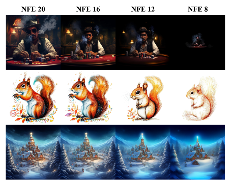
Figure 10 解读：附录的 sampling steps 可视化展示 teacher 在不同步数下预测 $x_{0}$ 的质量变化。步数增加让轨迹覆盖更细，通常改善中间 clean prediction；但当步数已经足够时，额外收益变小，因此最终需要在显存、训练时间和 FID 之间取舍。

$R$ 的 ablation 说明 loss 稳定项的最终权重不能简单沿用 sCM 的 1.0。固定 final $R$ 时，1.0 得到 FID 7.66、CLIP 28.00；0.75 最好，FID 6.77、CLIP 28.00；0.65 为 6.81/27.98；0.5 为 7.41/27.98。schedule 对比中，Warmup 得到 FID 6.58、CLIP 27.98，Warmup–Cooldown 得到 FID 6.48、CLIP 28.00。这表明 generation-space trajectory samples 改变了切向项的最佳尺度：先 warm up 到稳定训练，再 cooldown 到较小最终权重，可以避免不稳定项过强地支配优化。

论文的 limitation 主要来自 image-free 本身。TBCM 不使用真实图像监督（Without real image supervision），因此 student 的上限受 teacher capacity 和 teacher bias 限制；如果 teacher 的生成轨迹本身有缺陷，这些缺陷可能传给 student，表现为样本多样性受限或轻微 mode collapse。Brightness Filter 只能过滤异常暗的明显失败样本，无法保证所有语义偏差都被排除。另一个实践 caveat 是，released code 是在 Sana-Sprint/Sana 生态上实现的；虽然论文主张框架可迁移到其他 diffusion tasks，但迁移到其他 backbones 时需要重新处理时间参数化、teacher derivative、latent scaling、prompt encoder 成本和 generation-space sampling schedule。

总体来看，TBCM 的结果证明了一个清晰结论：continuous-time consistency distillation 的关键不只是 loss 形式，还包括样本空间的构造。把训练样本从 forward diffusion space 移到 teacher backward generation space，可以同时降低数据/VAE 依赖、减少训练成本，并改善 one-step distillation 质量。这使它在“Multimodal Generation / Acceleration & Distillation”分类下更像一种 distillation data/source redesign，而不是单纯采样器或模型结构改进。

Paper Notes

探索

Image-Free Timestep Distillation via Continuous-Time Consistency with Trajectory-Sampled Pairs

Image-Free Timestep Distillation via Continuous-Time Consistency with Trajectory-Sampled Pairs

1. Motivation (研究动机)

2. Idea (核心思想)

3. Method (方法)

3.1 预备公式：从 diffusion / flow 到 TrigFlow consistency

3.2 Trajectory-Backward Consistency：从 teacher ODE 收集训练对

3.3 Sampling scheme：generation space 中不仅要采样 timestep，还要采样 route

3.4 Brightness Filter：不解码图像也能过滤暗样本

3.5 Continuous-time consistency loss 与 $R$ 调整

3.6 Source-code mapping

4. Experimental Setup (实验设置)

5. Experimental Results (实验结果)

目录

Paper Notes

探索

Image-Free Timestep Distillation via Continuous-Time Consistency with Trajectory-Sampled Pairs

Image-Free Timestep Distillation via Continuous-Time Consistency with Trajectory-Sampled Pairs

1. Motivation (研究动机)

2. Idea (核心思想)

3. Method (方法)

3.1 预备公式：从 diffusion / flow 到 TrigFlow consistency

3.2 Trajectory-Backward Consistency：从 teacher ODE 收集训练对

3.3 Sampling scheme：generation space 中不仅要采样 timestep，还要采样 route

3.4 Brightness Filter：不解码图像也能过滤暗样本

3.5 Continuous-time consistency loss 与 R 调整

3.6 Source-code mapping

4. Experimental Setup (实验设置)

5. Experimental Results (实验结果)

目录

3.5 Continuous-time consistency loss 与 $R$ 调整