Live Avatar: Streaming Real-time Audio-Driven Avatar Generation with Infinite Length

Authors: Yubo Huang, Hailong Guo, Fangtai Wu, Shifeng Zhang, Shijie Huang, Qijun Gan, Lin Liu, Sirui Zhao, Enhong Chen, Jiaming Liu, Steven Hoi Affiliations: University of Science and Technology of China, Alibaba Group, Beijing University of Posts and Telecommunications, Zhejiang University arXiv: 2512.04677 Project Page: liveavatar.github.io GitHub: Alibaba-Quark/LiveAvatar

1. Motivation (研究动机)

实时性与质量的矛盾：现有基于 Diffusion 的视频生成模型（如 14B 参数的 DiT）虽然视觉质量卓越，但其顺序去噪的推理方式导致延迟极高，无法满足实时交互场景（≥20 FPS）的需求。现有实时方案（如 CausVid、LongLive）通过大幅缩减模型规模（1.3B）和激进量化来提速，但牺牲了生成质量。
长时序一致性问题：无限长度视频生成中，身份漂移（identity drift）、颜色偏移（color shift）和时序不稳定会随时间累积，严重影响 avatar 的视觉连贯性。现有方法在分钟级生成后质量显著退化。
算法-系统协同设计的缺失：目前尚无方法能同时实现 streaming、real-time、infinite-length 和 high-fidelity 四个目标，尤其是在大规模（14B）Diffusion 模型上。

Figure 1 解读：展示了 Live Avatar 的核心能力——支持实时 20 FPS（5 H800 GPU，4步采样）、流式 block-wise 自回归生成、超过 10000 秒的无限长度生成，以及对非人类角色（如火焰人）的泛化能力。输入为参考图像 + 音频 + 文本描述，输出为时间轴上持续生成的高保真 avatar 视频。

2. Idea (核心思想)

Live Avatar 的核心创新是算法-系统协同设计：在算法层面，通过 Self-Forcing Distribution Matching Distillation 将非因果教师模型蒸馏为因果少步学生模型，使其适配流式推理；在系统层面，提出 Timestep-forcing Pipeline Parallelism (TPP) 将顺序去噪步骤分配到不同 GPU 上并行执行，将吞吐量瓶颈从”所有去噪步之和”降低为”单次前向传播”。同时引入 Rolling Sink Frame Mechanism (RSFM) 解决长时序身份漂移问题。

与现有方法的根本区别：不是通过缩小模型来提速，而是通过分布式 pipeline 并行和蒸馏，在保持 14B 大模型质量的同时实现实时推理。

3. Method (方法)

3.1 整体框架

Live Avatar 的训练和推理框架分为两个阶段：

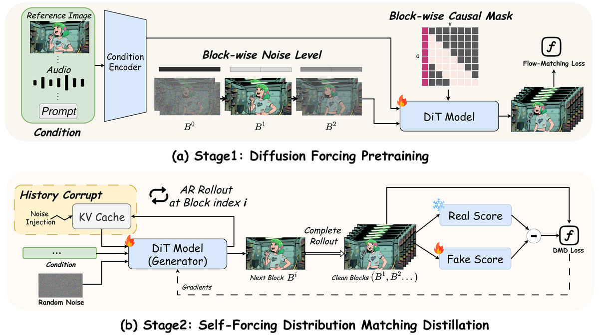
Figure 2 解读：(a) Stage 1: Diffusion Forcing Pretraining — 采用 block-wise 独立噪声调度和因果局部注意力掩码，将非因果模型适配为因果生成。输入包括 Reference Image、Audio 和 Prompt，经过 Condition Encoder 后，对 block $B^{0}, B^{1}, B^{2}$ 施加不同噪声级别，通过 block-wise causal mask（block 内部全连接，block 之间单向因果）送入 DiT 模型，用 Flow-Matching Loss 训练。(b) Stage 2: Self-Forcing Distribution Matching Distillation — 基于 Self-Forcing 范式，DiT Generator 自回归生成 block 序列，通过 History Corrupt（向 KV Cache 注入噪声）保持训练与推理的一致性。完整 rollout 的输出经 Real Score 和 Fake Score 网络计算 DMD Loss，蒸馏为少步（4步）生成器。

3.2 模型架构

模型基于 WanS2V（14B 参数的 DiT），采用 block-wise 自回归生成。每个 block 包含 3 帧 latent（对应物理帧数通过 VAE 的时间压缩比决定）。生成的联合分布被分解为：

B_{t - 1}^{i} = v_{θ} (B_{t}^{i}, kv cache B_{t}^{(i - w) : (i - 1)}, I, a^{i}, t^{i})

其中 $I$ 为 rolling sink frame（提供外观参考）， $a^{i}$ 和 $t^{i}$ 分别为第 $i$ 个 block 的音频和文本 embedding， $w$ 为 KV cache 窗口大小。关键设计：KV cache $B_{t}^{(i - w) : (i - 1)}$ 与当前 noisy block $B_{t}^{i}$ 共享相同噪声级别，这使得 timestep-forcing pipeline 并行成为可能。

3.3 训练流程

Stage 1: Diffusion Forcing Pretraining

使用 block-wise 独立噪声调度：每个 block 独立采样噪声级别
应用因果注意力掩码：block 内部全连接（intra-block full attention），block 之间单向因果（inter-block causal attention）
采用 Flow Matching 目标：

x_{t} = (1 - s_{t}) \cdot x_{0} + s_{t} \cdot x_{T}, s_{t} \in [0, 1]

目标速度： $v = x_{T} - x_{0}$

损失函数：

L = E_{x_{0}, x_{T}, t} [∥ v_{θ} (x_{t}, t, c) - (x_{T} - x_{0}) ∥_{2}^{2}]

Stage 2: Self-Forcing DMD with History Corrupt

基于 Distribution Matching Distillation (DMD) 进行少步蒸馏，包含三个关键模型：

Real Score Model（固定的双向教师模型）：提供目标分布
Fake Score Model（动态更新）：跟踪学生输出的分布
Causal Generator（因果学生模型）：从 Stage 1 初始化，优化为少步生成

DMD 梯度：

\nabla_{θ} L_{DMD} = - E_{t, z} [(s_{real} (x_{t}, t) - s_{fake, ϕ} (x_{t}, t)) \cdot \frac{\partial G _{θ} ( z )}{\partial θ}]

History Corrupt 机制：在训练时向 KV cache 注入随机噪声，使模型学会区分来自历史帧的动态运动信息和 sink frame 的静态身份特征。这弥合了训练（clean cache）和推理（noisy cache）之间的 gap。

Block-wise Gradient Accumulation：由于 DMD 训练显存需求巨大，采用分 block 反向传播 + 梯度累积策略，在保持训练行为一致的同时显著降低峰值显存。

# Stage 1: Diffusion Forcing pretraining
while not converged:
    x0 = sample_video_clip(dataset)
    blocks = partition_video(x0, block_size=3)
 
    noisy_blocks = []
    timesteps = []
    noises = []
    for block in blocks:
        t = uniform(0.0, 1.0)                 # 每个 block 独立采样噪声级别
        eps = gaussian_like(block)
        block_t = (1 - t) * block + t * eps
 
        noisy_blocks.append(block_t)
        timesteps.append(t)
        noises.append(eps)
 
    mask = build_blockwise_causal_mask(num_blocks=len(blocks))
    v_pred = v_theta(noisy_blocks, timesteps, conditions, mask=mask)
 
    loss = 0.0
    for i, block in enumerate(blocks):
        target = noises[i] - block           # flow-matching target
        loss += squared_l2(v_pred[i], target)
 
    optimize(loss, params=theta)

# Self-Forcing DMD with History Corrupt
T = len(timesteps)
 
while not converged:
    x_theta = []
    kv_cache = []
    s = randint(0, T - 1)                    # 随机选择一个需要反传的 timestep
 
    for frame_idx in range(N):
        x_t = gaussian_latent()
 
        for step_idx in range(T - 1, s - 1, -1):
            t = timesteps[step_idx]
 
            if step_idx == s:
                with grad_enabled():
                    kv_i, x0_hat = G_theta.kv_forward(x_t, t, kv_cache, conditions[frame_idx])
                x_theta.append(x0_hat)
                kv_cache.append(detach(kv_i))   # History Corrupt: noisy KV cache
            else:
                with no_grad():
                    x0_hat = G_theta(x_t, t, kv_cache, conditions[frame_idx])
                eps = gaussian_like(x_t)
                x_t = psi(x0_hat, eps, timesteps[step_idx - 1])
 
    loss = dmd_loss(x_theta)
    optimize(loss, params=theta)

# Block-wise gradient accumulation for DMD training
T = len(timesteps)
 
while not converged:
    x_theta = []
    x_cache = []
    kv_cache = []
    s = randint(0, T - 1)
 
    # Phase 1: rollout without gradient
    with no_grad():
        for frame_idx in range(N):
            x_t = gaussian_latent()
 
            for step_idx in range(T - 1, s - 1, -1):
                t = timesteps[step_idx]
 
                if step_idx == s:
                    kv_i, x0_hat = G_theta.kv_forward(x_t, t, kv_cache, conditions[frame_idx])
                    x_cache.append(detach(x_t))  # 保存 x_{t_s} 供 replay
                    x_theta.append(detach(x0_hat))
                    kv_cache.append(detach(kv_i))
                else:
                    x0_hat = G_theta(x_t, t, kv_cache, conditions[frame_idx])
                    eps = gaussian_like(x_t)
                    x_t = psi(x0_hat, eps, timesteps[step_idx - 1])
 
    # Phase 2: replay one block at a time with gradient
    for frame_idx in reversed(range(N)):
        partial_outputs = []
 
        for j in range(N):
            if j == frame_idx:
                with grad_enabled():
                    x0_hat = G_theta(x_cache[j], timesteps[s], kv_cache, conditions[j])
                partial_outputs.append(x0_hat)
            else:
                partial_outputs.append(x_theta[j])
 
        loss = dmd_loss(partial_outputs)
        loss.backward()
        kv_cache.pop()                         # 逆序释放 KV，控制峰值显存
 
    optimizer.step()
    optimizer.zero_grad()

3.4 Timestep-forcing Pipeline Parallelism (TPP)

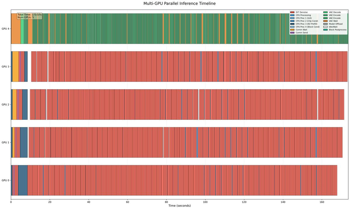
Figure 3 解读：TPP 的核心思想是将 4 步去噪的顺序执行转化为跨 GPU 的流水线并行。左侧展示了 warmup 阶段（第一个 block 填充 pipeline），之后进入 fully pipelined streaming 阶段——所有 GPU 同时处理不同 block 的不同 timestep。例如：GPU0 处理 $t_{4} \to t_{3}$ ，GPU1 处理 $t_{3} \to t_{2}$ ，GPU2 处理 $t_{2} \to t_{1}$ ，GPU3 处理 $t_{1} \to t_{0}$ ，GPU4 负责 VAE decode。右侧说明了通信方式：GPU 内复用本地 KV Cache（Very Fast），GPU 间仅传递 latent（Fast），而不传递 KV Cache（Slow，被避免）。

TPP 的关键设计：

每个 GPU 固定一个 timestep： $GP U_{k}$ 始终执行 $t_{k} \to t_{k - 1}$ 的变换
Warmup 阶段：第一个 block 依次通过所有 GPU 填充 pipeline
Fully pipelined 阶段：每个 GPU 完成当前 block 后，将 latent 传给下一个 GPU，立即处理新 block
KV Cache 完全本地化：每个 GPU 仅使用自己 timestep 的 KV cache，无需跨 GPU 传输（因为 KV cache 与当前 block 共享噪声级别）
VAE Decode 独立 GPU：防止解码成为 pipeline 瓶颈

吞吐量由单次模型前向传播决定，而非所有去噪步之和：

FPS = \frac{frames_per_block}{single_forward_time}

# TPP multi-GPU inference with AAS and Rolling RoPE
def tpp_inference(gpu_idx, timesteps, max_kv, num_frames, conditions, ref_image):
    T = len(timesteps)
    video = []
    kv_cache = []
    sink = ref_image
    dt = -1.0 / T
 
    for frame_idx in range(num_frames):
        if gpu_idx == 0:
            x_t = gaussian_latent()            # 第一个 DiT 设备负责采样初始噪声
        else:
            x_t = dist.recv()
 
        if gpu_idx == T:
            frame = vae_decode(x_t)            # 最后一张卡专门做 VAE decode
            video.append(frame)
 
            if frame_idx == 0:
                sink = frame                   # AAS: 用首帧更新 sink
                dist.broadcast(sink)
            continue
 
        if frame_idx == 1:
            sink = dist.recv()                 # AAS: 接收首帧作为新的 sink
 
        step_idx = T - 1 - gpu_idx
        v_pred, kv_i = v_theta.kv_forward(
            x_t,
            timesteps[step_idx],
            kv_cache,
            conditions[frame_idx],
            rope=rolling_rope(sink),
        )
 
        if len(kv_cache) == max_kv:
            kv_cache.pop(0)
        kv_cache.append(kv_i)
 
        x_t = x_t + dt * v_pred
        dist.send(x_t)
 
    return video

3.5 Rolling Sink Frame Mechanism (RSFM)

长时序生成面临两类漂移问题：

Figure 6 解读：对比四种推理设置。(a) Baseline：使用固定 sink frame 和标准 rolling-kv-cache，KV cache 通过虚线箭头传递。(b) with AAS：将 sink 替换为第一个生成帧（红色标记），解决 distribution drift。(c) with Timestep-Forcing：每个 noisy latent 仅关注相同 timestep 的 KV cache（绿色标记），实现 pipeline 并行。(d) Ours：结合 AAS 和 timestep-forcing 的完整方案。

Adaptive Attention Sink (AAS)

解决 distribution drift 问题：原始 sink frame（参考图像的 VAE 编码）来自真实图像分布，但生成帧来自模型的学习分布，两者存在系统性偏差。AAS 在生成第一个 block 后，用模型自己生成的第一帧替换原始 sink frame，使后续所有 block 的条件都来自模型分布内部，抑制分布漂移。

Rolling RoPE

解决 inference-mode drift 问题：sink frame 与当前 block 之间的 RoPE 相对位置会随生成长度线性增长，远超训练分布。Rolling RoPE 动态调整 sink frame 的 RoPE 位置，使其始终保持在当前 block 之前固定距离，确保相对位置编码落在训练分布内。

Figure 7 解读：Rolling RoPE 的可视化。每个矩形内的数字表示 block index 和 RoPE index。随着自回归 rollout 进行，每次 RoPE Update 时 sink frame (B1) 的 RoPE index 动态递增（ $R_{k}, R_{1 + k}, R_{2 + k} ...$ ），保持 sink frame 的 RoPE index 始终略大于当前 noisy block，确保全程维持稳定的相对位置距离。

# Single-GPU inference with AAS and Rolling RoPE
def single_gpu_inference(timesteps, max_kv, num_frames, conditions, ref_image):
    video = []
    kv_caches = [[] for _ in timesteps]        # 每个 timestep 单独维护 KV cache
    sink = ref_image
    dt = -1.0 / len(timesteps)
 
    for frame_idx in range(num_frames):
        x_t = gaussian_latent()
 
        for step_idx in reversed(range(len(timesteps))):
            v_pred, kv_i = v_theta.kv_forward(
                x_t,
                timesteps[step_idx],
                kv_caches[step_idx],
                conditions[frame_idx],
                rope=rolling_rope(sink),
            )
            x_t = x_t + dt * v_pred
 
            if len(kv_caches[step_idx]) == max_kv:
                kv_caches[step_idx].pop(0)
            kv_caches[step_idx].append(kv_i)
 
        frame = vae_decode(x_t)
        video.append(frame)
 
        if frame_idx == 0:
            sink = x_t                          # AAS: 改用模型生成的首帧 latent
 
    return video

3.6 Code-to-Paper 映射表

Paper Concept	Source File	Key Class/Function
因果 DiT 模型	`liveavatar/models/wan/causal_model_s2v.py`	`CausalWanModel_S2V`, `CausalWanS2VSelfAttention`
Block-wise Causal Mask	`liveavatar/models/wan/causal_model_s2v.py`	`_prepare_blockwise_causal_attn_mask()`
Single-GPU Pipeline	`liveavatar/models/wan/causal_s2v_pipeline.py`	`WanS2V.generate()`
TPP Multi-GPU Pipeline	`liveavatar/models/wan/causal_s2v_pipeline_tpp.py`	`WanS2VTPP` pipeline, `dist.send()`/`dist.recv()` for latent passing
Rolling KV Cache	`liveavatar/models/wan/causal_model_s2v.py`	`_initialize_kv_cache()`, circular buffer via `current_start % kv_cache_size`
AAS (Adaptive Attention Sink)	`liveavatar/models/wan/causal_s2v_pipeline_tpp.py`	`ref_latents = block_latents[:,:,0:1]` at block_index=0
Rolling RoPE	`liveavatar/models/wan/causal_model_s2v.py`	`rope_precompute()`, `freqs_cond` with dynamic offset
History Corrupt	`liveavatar/models/wan/causal_model_s2v.py`	`trainable_cond_mask` embedding, noise injection into KV
S2V Model Config	`liveavatar/models/wan/wan_2_2/modules/s2v/model_s2v.py`	S2V model definition
Scheduler	`liveavatar/scheduler.py`	`SchedulerInterface`, X0/noise/velocity conversions
Gradio Demo	`minimal_inference/gradio_app.py`	Web UI for inference

4. Experimental Setup (实验设置)

数据集

训练集：AVSpeech 数据集，经过 OmniAvatar 的预处理流程过滤（仅保留 >10s 的片段），最终得到 400,000 个高质量样本
测试集 GenBench：使用 Gemini-2.5 Pro、Qwen-Image、CosyVoice 合成生成，包含：
- GenBench-ShortVideo：100 个约 10 秒的测试样本
- GenBench-LongVideo：15 个超过 5 分钟的测试视频
- 涵盖写实人类、动画角色、拟人化非人类，正面和侧面视角
In-domain 测试：从 AVSpeech 中抽取 5% 的 50 个片段（5-10s）

Baselines

Ditto (0.2B), EchoMimic-V2, Hallo3 (5B), StableAvatar (1.3B), OmniAvatar (14B), WanS2V (14B)

评估指标

图像质量：FID, FVD
感知质量：ASE↑（Q-align 美学分数）, IQA↑（Q-align 图像质量）
音视频同步：Sync-C↑, Sync-D↓
语义一致性：Dino-S↑（DINOv2 相似度）
效率：FPS↑, TTFF↓（Time-to-First-Frame）

训练配置

硬件：128 NVIDIA H800 GPUs
分辨率：720×400，84 帧
训练步数：Stage 1: 25K steps, Stage 2: 2.5K steps（共约 500 GPU days）
Batch size：per-GPU batch size = 1，使用 FSDP + gradient accumulation
学习率：Student 1e-5, Fake Score 2e-6
Block 设置：每 3 帧一个 block，KV cache 长度 4 blocks，单个 rolling sink frame
LoRA：rank=128, alpha=64

5. Experimental Results (实验结果)

主要性能对比

GenBench-ShortVideo (10s):

Model	ASE↑	IQA↑	Sync-C↑	Sync-D↓	Dino-S↑	FPS↑
Ditto	3.31	4.24	4.09	10.76	0.99	21.80
Hallo3	3.12	3.97	4.74	10.19	0.94	0.26
StableAvatar	3.52	4.47	3.42	11.33	0.93	0.64
OmniAvatar	3.53	4.49	6.77	8.22	0.93	0.16
WanS2V	3.36	4.29	5.89	9.08	0.95	0.25
Ours	3.44	4.35	5.69	9.13	0.95	20.88

GenBench-LongVideo (7min):

Model	ASE↑	IQA↑	Sync-C↑	Sync-D↓	Dino-S↑	FPS↑
OmniAvatar	2.36	2.86	8.00	7.59	0.66	0.16
WanS2V	2.63	3.99	6.04	9.12	0.80	0.25
Ours	3.38	4.73	6.28	8.81	0.94	20.88

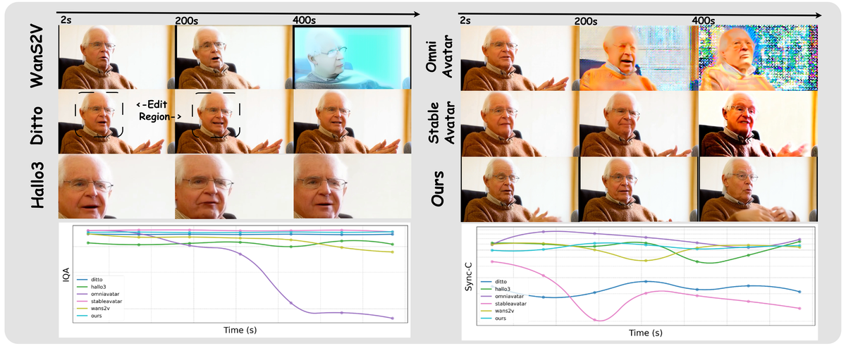
Figure 4 解读：长视频生成的定性对比。左右两组分别展示两个不同角色在 2s、200s、400s 时间点的生成帧。WanS2V 和 Ditto 在长时间后出现明显的画质退化和身份漂移（如 Ditto 的 Edit Region 标注区域），OmniAvatar 和 StableAvatar 也出现颜色偏移。Live Avatar（Ours）在整个序列中保持稳定的身份和高画质。下方的 IQA 和 Sync-C 曲线图显示 Live Avatar 的指标随时间保持平稳，而其他方法逐渐下降。

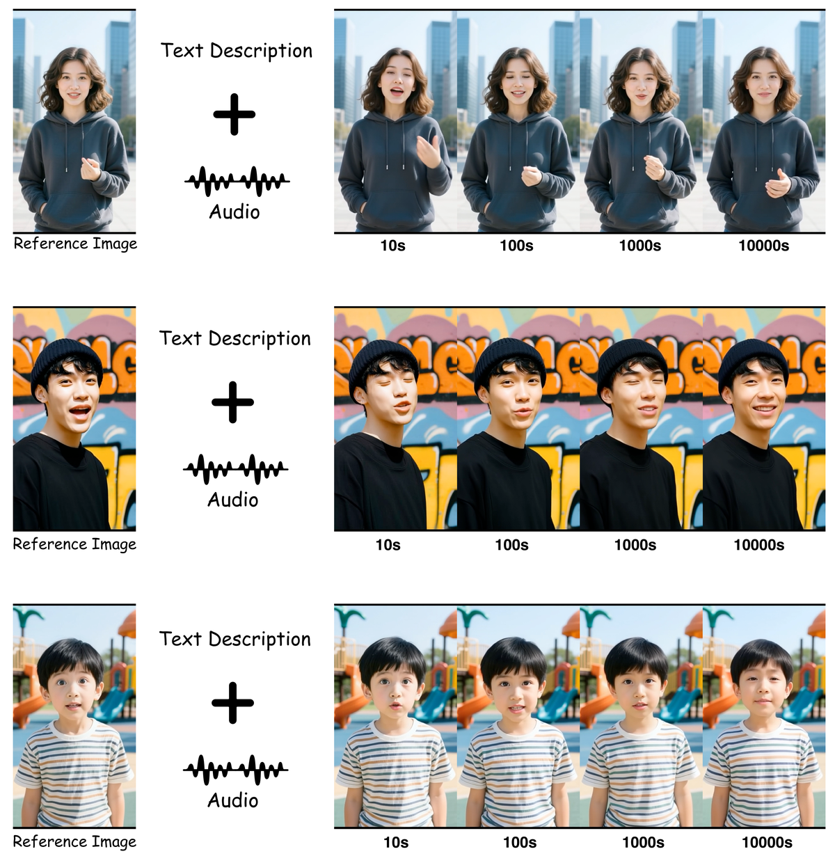
Figure 5 解读：GenBench-ShortVideo 上的定性对比。展示了 reference image 与 Live Avatar（Ours）、OmniAvatar、EchoMimic-V2 的生成结果。Live Avatar 在保真度和自然度上均表现最优，OmniAvatar 在某些角色上出现不自然的姿态，EchoMimic-V2 因依赖固定骨骼模板导致面部变形。

关键发现：

Live Avatar 在长视频场景下优势更为显著，ASE 和 IQA 大幅领先所有 baseline
FPS 达到 20.88，相比最快的 baseline Ditto（21.80 FPS, 0.2B）仅略低，但质量远超
长视频中其他方法的 Dino-S 显著下降（OmniAvatar: 0.93→0.66），Live Avatar 保持稳定（0.95→0.94）

推理效率消融 (Table 3)

Methods	GPUs	NFE	FPS↑	TTFF↓
w/o TPP	2	5	4.26	3.88
w/o TPP, w/ SP_4GPU	5	5	5.01	3.24
w/o VAE Parallel	4	4	10.16	4.73
w/o DMD	2	80	0.29	45.50
Ours	5	4	20.88	2.89

DMD 蒸馏贡献最大（80步→4步），TPP 实现 pipeline 并行（4.26→20.88 FPS）
序列并行（SP）仅提供边际增益，因 block 序列长度短，通信开销抵消了并行收益
VAE 独立 GPU 解码消除了 pipeline 瓶颈

Rolling Sink Frame 消融 (Table 4, Long Video)

Methods	ASE↑	IQA↑	Sync-C↑	Dino-S↑
w/o AAS	3.13	4.44	6.25	0.91
w/o Rolling RoPE	3.38	4.71	6.29	0.86
w/o History Corrupt	2.90	3.88	6.14	0.81
Ours	3.38	4.73	6.28	0.93

History Corrupt 对质量影响最大（IQA 下降 0.85）
Rolling RoPE 对身份一致性（Dino-S）至关重要（0.93→0.86）
注：Table 4 中完整模型 Dino-S 为 0.93，Table 2 主实验为 0.94，差异源于 Table 4 使用不同的长视频评估子集

10,000 秒超长生成 (Table 7)

Time Segment	ASE↑	IQA↑	Sync-C↑	Dino-S↑
0-10s	3.37	4.72	6.20	0.94
100-110s	3.38	4.71	6.44	0.93
1000-1010s	3.37	4.69	5.98	0.93
10000-10010s	3.38	4.71	6.26	0.93

各指标在 10000 秒时间跨度内几乎无退化，证明 RSFM 的有效性

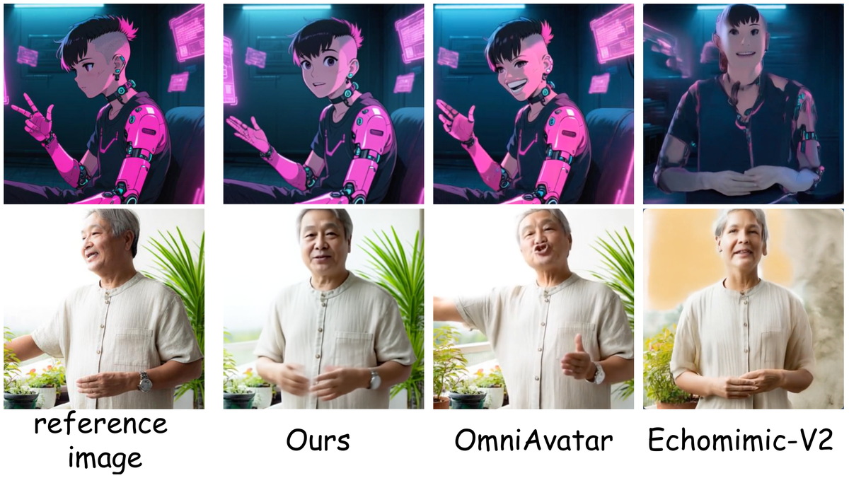
Figure 8 解读：Multi-GPU Parallel Inference Timeline，展示 5 个 GPU（GPU 0-4）的计算和等待时间分布。左侧两段白色间隙为 warmup 阶段（包括 AAS 的二次 warmup）。此后大部分时间被红色的 DiT 计算占据，显示各 GPU 利用率高且帧率稳定。偶尔出现的白色间隙（idle time）由帧率波动引起，对整体性能影响可忽略。

用户研究 (Table 5)

Model	Naturalness↑	Synchronization↑	Consistency↑
Ditto	78.2	40.5	90.2
OmniAvatar	71.1	78.5	90.8
WanS2V	84.3	85.2	92.0
Ours	86.3	80.6	91.1

Live Avatar 在 Naturalness 上最优，在三项指标上最为均衡
OmniAvatar 虽然客观 Sync-C 最高，但人类评估的同步性仅 78.5，说明过度优化唇动反而损害自然感

局限性

TPP 提升 FPS 但不降低 TTFF（首帧延迟），限制交互响应性
对 RSFM 的强依赖在复杂场景下可能影响长期时序一致性

Paper Notes

探索

Live Avatar: Streaming Real-time Audio-Driven Avatar Generation with Infinite Length

Live Avatar: Streaming Real-time Audio-Driven Avatar Generation with Infinite Length

1. Motivation (研究动机)

2. Idea (核心思想)

3. Method (方法)

3.1 整体框架

3.2 模型架构

3.3 训练流程

Stage 1: Diffusion Forcing Pretraining

Stage 2: Self-Forcing DMD with History Corrupt

3.4 Timestep-forcing Pipeline Parallelism (TPP)

3.5 Rolling Sink Frame Mechanism (RSFM)

Adaptive Attention Sink (AAS)

Rolling RoPE

3.6 Code-to-Paper 映射表

4. Experimental Setup (实验设置)

数据集

Baselines

评估指标

训练配置

5. Experimental Results (实验结果)

主要性能对比

推理效率消融 (Table 3)

Rolling Sink Frame 消融 (Table 4, Long Video)

10,000 秒超长生成 (Table 7)

用户研究 (Table 5)

局限性

目录