AnyFlow: Any-Step Video Diffusion Model with On-Policy Flow Map Distillation

Paper: arXiv:2605.13724 PDF: arXiv PDF；local: /Users/bytedance/ai-skills/papers/2605.13724.pdf Code: NVlabs/AnyFlow Code reference: main @ 549236a (2026-05-14)

1. Motivation（研究动机）

现有少步视频扩散蒸馏主要依赖 consistency model：它在很少采样步数时很快，但训练目标偏向端点映射 ${\mathbf{z}}_t\to {\mathbf{z}}_0$。当推理时给更多 NFE，模型会反复把中间状态 re-noise 再投影到端点，轨迹不再沿原始 probability-flow ODE 稳定 refinement，因此 rCM / Self-Forcing 这类方法会出现“步数越多质量反而下降”的 test-time scaling 失败。

AnyFlow 的核心问题定义是：能否训练一个单一视频扩散模型，让它在任意推理步数下都可用，并且随采样预算增加继续变好，而不是只为固定 1/2/4 步做蒸馏。它把目标从端点一致性改为任意时间对之间的 flow-map transition：

$$\frac{d{\mathbf{z}}_t}{dt}=\mathbf{v}({\mathbf{z}}_t,t),{\mathbf{f}}_{\theta }({\mathbf{z}}_t,t,r)\approx {\mathbf{z}}_r,1\ge t>r\ge 0.$$

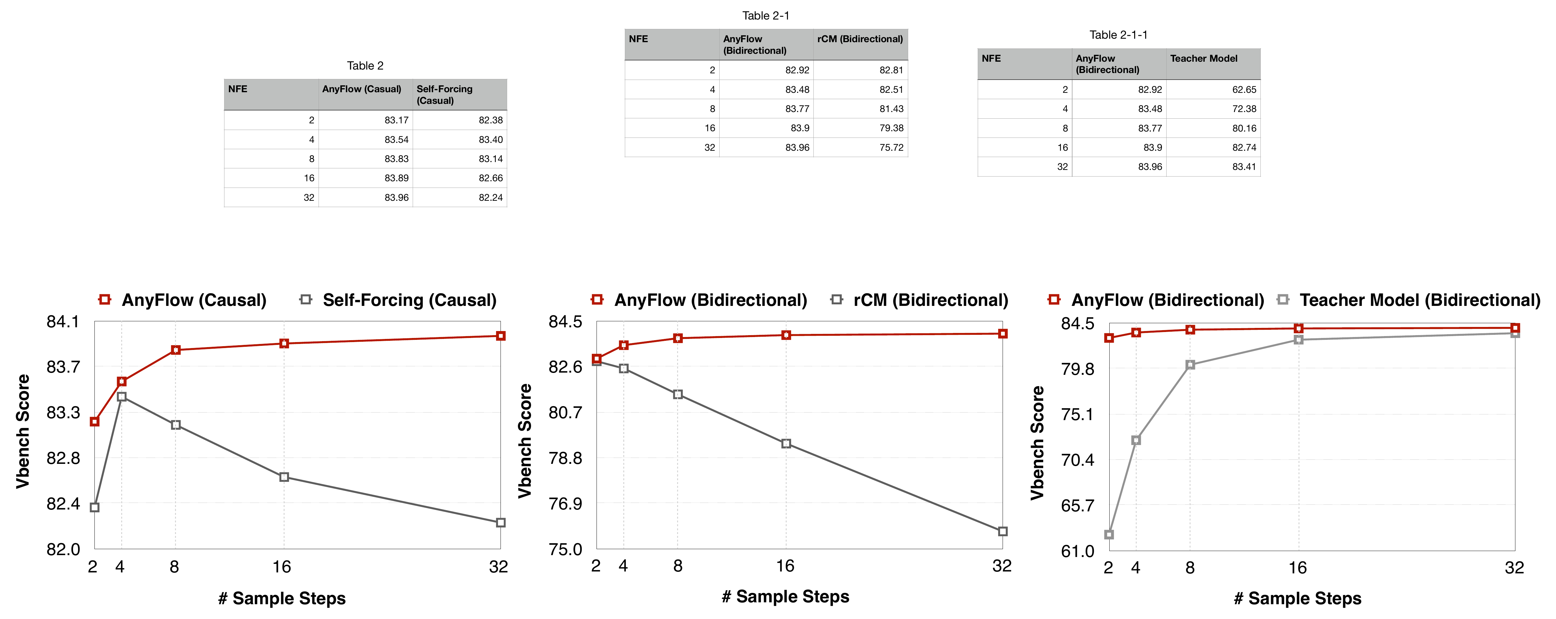
Figure 1 解读：AnyFlow 在 causal、bidirectional、teacher-distilled 三组曲线上都保持随采样步数增加而上升或基本不退化；对照方法 Self-Forcing 和 rCM 在多步时明显下滑，说明问题不是“少步不够好”，而是 consistency trajectory 与 PF-ODE trajectory 的结构性偏移。

本文贡献可以压缩成三点：第一，提出首个基于 flow maps 的 any-step video diffusion distillation 框架；第二，提出 Flow Map Backward Simulation，把 on-policy DMD 所需的自回放轨迹拆成可反传的 shortcut transition；第三，在 1.3B/14B、bidirectional/causal、T2V/I2V/V2V 设置上验证任意步数扩展性。

2. Idea（核心思想）

AnyFlow 的核心 insight 是：少步视频扩散蒸馏不应该只学习“任意噪声时刻到干净样本”的 endpoint consistency，而应该学习任意两个时间点之间可组合的 flow-map transition。这样同一个 student 在 1-step / 2-step / 4-step / 多步推理时共享同一套 transition 语义，采样步数增加时仍能沿 teacher ODE 轨迹继续 refinement。

关键创新可以概括为两点：第一，用 forward flow map training 把 teacher probability-flow ODE 上的跨时间迁移显式蒸馏出来；第二，用 on-policy flow map distillation 在 student 自己 roll out 的状态分布上继续校正，避免 student 一旦偏离 teacher 轨迹后误差累积。

与 rCM / shortcut consistency 这类 endpoint-oriented 方法相比，AnyFlow 的本质差异是优化对象从 ${\mathbf{z}}_{t}ightarrow{\mathbf{z}}_0$ 的端点映射变成 ${\mathbf{z}}_{t}ightarrow{\mathbf{z}}_r$ 的时间迁移算子。前者适合固定少步采样，后者天然支持任意 step budget 下的分段组合，因此更适合 video diffusion 中“速度—质量可调”的部署场景。

3. Method（方法）

3.1 从 consistency distillation 到 flow-map distillation

Consistency distillation 学的是“从任意 $t$ 回到 $0$”，多步推理时需要反复 re-noise；AnyFlow 学的是“从 $t$ 到任意较小 $r$”，因此同一个模型既可以执行大步 shortcut，也可以在更多 NFE 下做小步 refinement。采样器在 released code 中直接实现为：

$${\mathbf{z}}_r={\mathbf{z}}_t-(t-r){\mathbf{u}}_{\theta }({\mathbf{z}}_t,t,r).$$

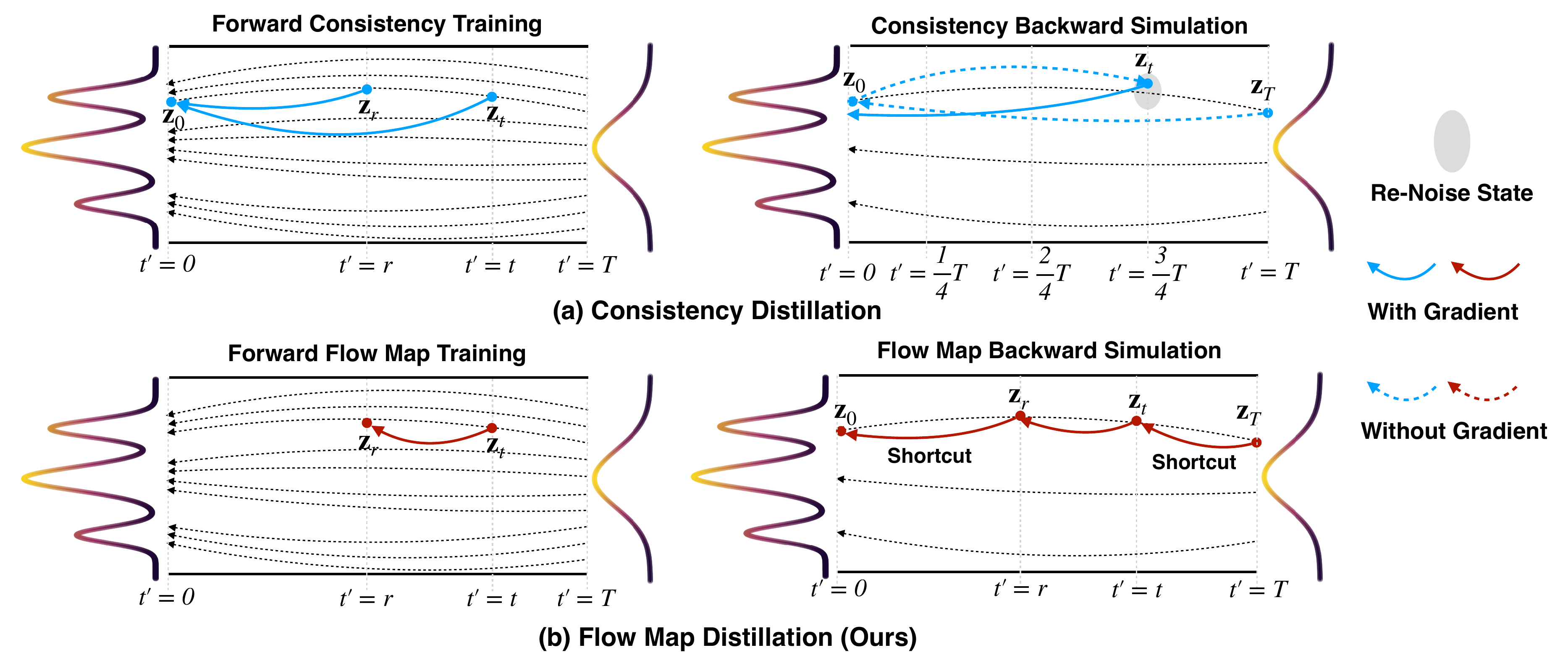
Figure 2 解读：上半部分的 consistency 路线把多个状态都拉向 ${\mathbf{z}}_0$，再经 re-noise 进入下一个状态；下半部分的 AnyFlow 直接学习 ${\mathbf{z}}_t\to {\mathbf{z}}_r$ transition，并在 backward simulation 中用 $T\to t\to r\to 0$ 的 shortcut 保留梯度链路。

3.2 整体训练流水线

AnyFlow 两阶段训练：Stage 1 做 forward flow map training，用 teacher-synthesized 数据把 Wan2.1 类视频扩散模型改造成 transition operator；Stage 2 从 Stage-1 checkpoint 出发，联合 forward objective 与 DMD-based on-policy objective，用 teacher 的 distribution matching 纠正自回放轨迹中的 discretization error 与 causal exposure bias。

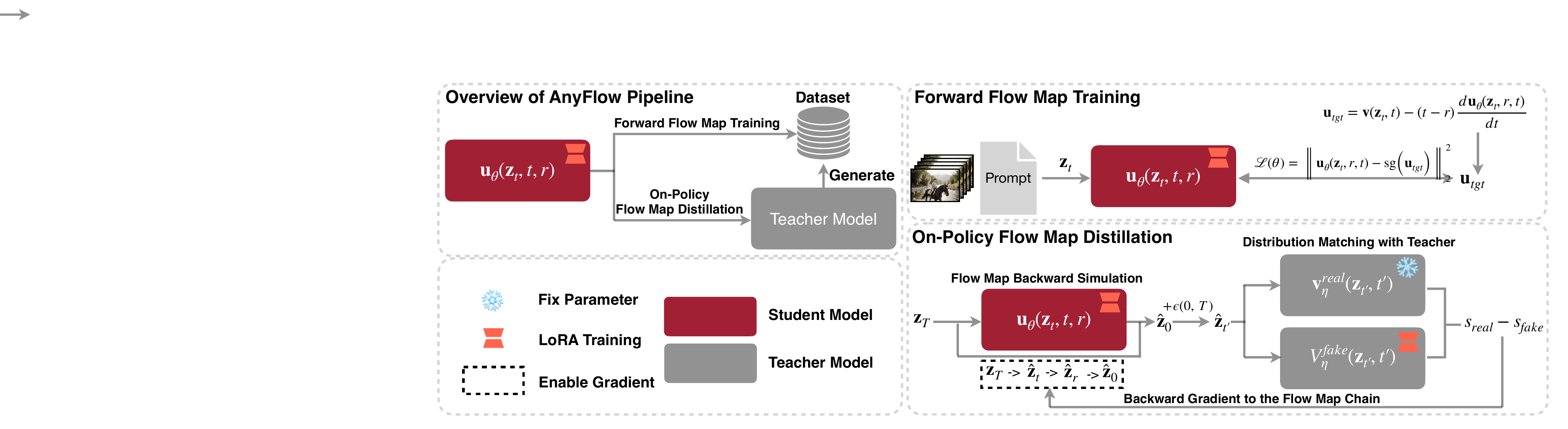
Figure 4 解读：左侧是数据生成与 LoRA student/teacher 参数冻结关系；右上是 forward flow map training，把 prompt/video/noise 时间对送入 student 预测 transition velocity；右下是 on-policy distillation，student 先通过 flow-map chain rollout 到 ${\hat{\mathbf{z}}}_0$，再 re-noise 给 real/fake teacher score 做 DMD 梯度监督。

3.3 Forward Flow Map Training

基础目标沿用 MeanFlow 风格：模型预测平均速度 ${\mathbf{u}}_{\theta }$，目标速度由瞬时 velocity 与导数校正构成：

$$\mathcal{L}(\theta )=\mathbb{E}\left[{\Vert {\mathbf{u}}_{\theta }({\mathbf{z}}_t,r,t)-\mathrm{sg}({\mathbf{u}}_{\text{tgt}})\Vert }_2^2\right],$$ $${\mathbf{u}}_{\text{tgt}}=\mathbf{v}({\mathbf{z}}_t,t)-(t-r)\frac{d{\mathbf{u}}_{\theta }({\mathbf{z}}_t,r,t)}{dt}.$$

为避免 JVP 与 FSDP 兼容/开销问题，AnyFlow 使用中心差分近似：

$$\frac{d}{dt}\mathbf{u}({\mathbf{z}}_t,r,t)\approx \frac{\mathbf{u}({\mathbf{z}}_{t+\Delta t},r,t+\Delta t)-\mathbf{u}({\mathbf{z}}_{t-\Delta t},r,t-\Delta t)}{2\Delta t}.$$

两个工程化细节很关键：

• Interpolated timestep conditioning：用 $g\cdot \mathrm{emb}(t)+(1-g)\cdot {\mathrm{emb}}^{\prime }(r)$ 引入第二时间 $r$，paper 和 released config 均使用 $g=0.25$，避免 zero-init 新 embedding 在训练中 norm 爆涨导致过饱和。
• Guidance-fused training：把 CFG 融进预测而不是 target velocity：

$$\mathbf{u}=\frac{1}{g}\left({\mathbf{u}}_c-(1-g)\mathrm{sg}({\mathbf{u}}_{\varnothing })\right).$$

• Loss reweighting：对非边界 transition 使用

$$w_{t,r}=\{\begin{array}{ll}1,& t=r\\ \frac{{\mu }_{t=r}}{\Vert \Delta {\Vert }_2^2+c},& t\ne r\end{array}$$

其中 ${\mu }_{t=r}$ 来自边界样本的平均 regression loss；实验固定 $w(t)=\mathrm{Beta}(2,1.5)$。

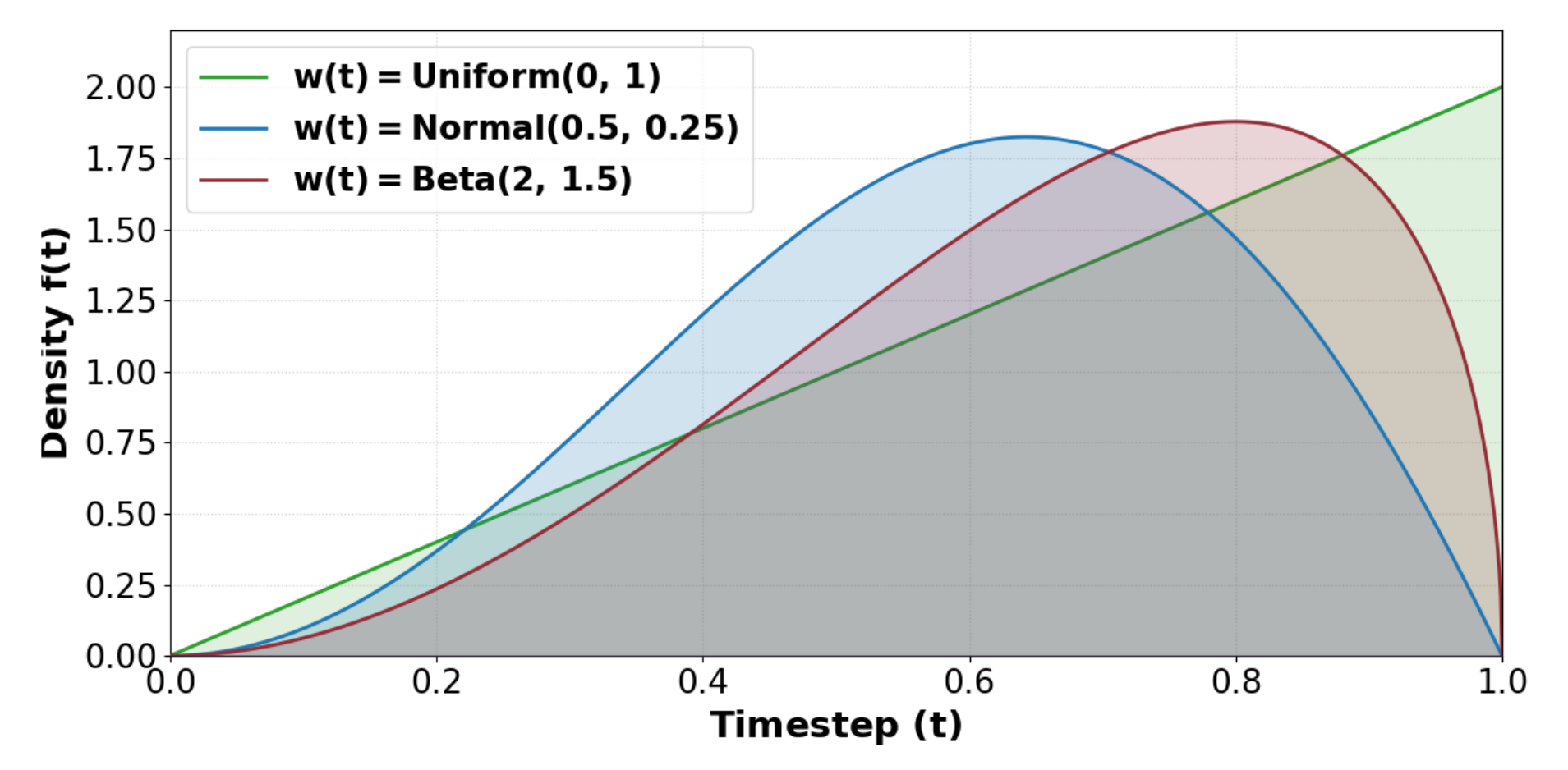
Figure 10 解读：不同 timestep weighting 会改变少步与多步的折中；作者最终选 Beta(2,1.5)，让训练更多覆盖高噪声但不完全牺牲低噪声区域，从而稳定 4/32 NFE 两端的 VBench。

3.4 On-Policy Flow Map Distillation

Forward training 只让 transition operator 拟合 teacher/ODE 的局部关系，仍然没有直接优化“模型自己按推理 scheduler rollout 后会落到哪里”。Stage 2 用 DMD 在 student self-rollout 上做 reverse-divergence correction。Flow map 的可组合性是关键：

$${\mathbf{f}}_{\theta }({\mathbf{z}}_t,t,q)\approx {\mathbf{f}}_{\theta }({\mathbf{f}}_{\theta }({\mathbf{z}}_t,t,r),r,q),t>r>q.$$

对于目标采样预算 $N$，AnyFlow 采样中间 $t$ 并令 $t-r=T/N$，把完整 $T\to 0$ rollout 拆为 $T\to t$、$t\to r$、$r\to 0$ 三段；第一和第三段可用 learned flow map shortcut，第二段是目标 gradient step。这样训练不同 NFE 的 self-rollout 时计算量基本不随 $N$ 线性增长。

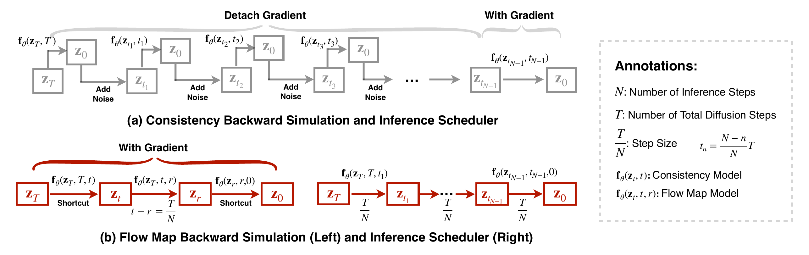
Figure 5 解读：consistency backward simulation 为了到达 ${\mathbf{z}}_0$ 往往截断较长 rollout 的梯度；flow-map simulation 只用三段 transition 就能覆盖同一个 training target，并把梯度回传到整条 shortcut chain，因此在 16/32 NFE 下不会像 consistency simulation 一样退化。

3.5 下游与 causal/bidirectional 适配

Bidirectional 版本直接套用上述两阶段；causal 版本接入 FAR pipeline：保留前三个 full-token chunks，后续 chunks 用更大 patchify kernel 压缩，以降低 teacher-forcing 训练成本和采样 KV cache。一个 causal AnyFlow-FAR 模型同时支持 T2V、I2V、V2V；I2V 通过 conditioning 首帧，V2V 通过下游 fine-tuning 使用 source video 的 compact context。

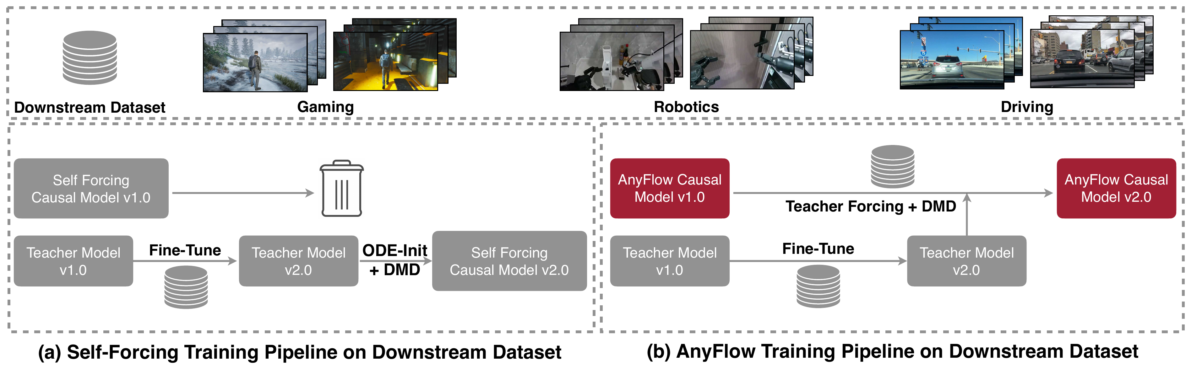
Figure 7 解读：下游 fine-tuning 不重新设计 distillation 目标，而是在 causal context 中加入 image/video 条件，把同一个 any-step transition operator 迁移到 I2V/V2V；这也是 AnyFlow 能用一个 FAR backbone 覆盖多任务的原因。

3.6 伪代码（按 released code 对齐）

import torch
import torch.nn.functional as F
 
 
def flowmap_euler_step(sample, model_output, t, r, num_train_timesteps=1000):
    # far/schedulers/scheduling_flowmap_euler_discrete.py
    t = t / num_train_timesteps
    r = r / num_train_timesteps
    while t.ndim < model_output.ndim:
        t = t[..., None]
        r = r[..., None]
    return sample - (t - r) * model_output

def forward_flow_map_pretrain_step(transformer, scheduler, latents, noise, prompt_embeds,
                                   neg_embeds, cfg_scale=3.0, eps=5, diffusion_ratio=0.5,
                                   consistency_ratio=0.25):
    # far/trainers/trainer_wan_anyflow_pretrain.py
    b = latents.shape[0]
    t1, t2 = torch.rand(b, device=latents.device), torch.rand(b, device=latents.device)
    t, r = torch.maximum(t1, t2), torch.minimum(t1, t2)
 
    # released sampler mixes boundary diffusion, consistency, and arbitrary flow-map transitions
    n_diff = round(diffusion_ratio * b)
    n_cons = round(consistency_ratio * b)
    r[:n_diff] = t[:n_diff]       # diffusion boundary: t == r
    r[n_diff:n_diff+n_cons] = 0   # consistency boundary: r == 0
 
    t = scheduler.apply_shift(t) * scheduler.config.num_train_timesteps
    r = scheduler.apply_shift(r) * scheduler.config.num_train_timesteps
    noisy = scheduler.scale_noise(latents, t, noise)
    v = noise - latents
 
    u_c = transformer(noisy, timestep=t, r_timestep=r, encoder_hidden_states=prompt_embeds)[0]
    with torch.no_grad():
        u_empty = transformer(noisy, timestep=t, r_timestep=r, encoder_hidden_states=neg_embeds)[0]
    u = (u_c - (1 - cfg_scale) * u_empty.detach()) / cfg_scale
 
    z_plus = noisy + v * (eps / scheduler.config.num_train_timesteps)
    z_minus = noisy - v * (eps / scheduler.config.num_train_timesteps)
    du_dt = (transformer(z_plus, t + eps, r, prompt_embeds)[0]
             - transformer(z_minus, t - eps, r, prompt_embeds)[0]) / (2 * eps)
    u_tgt = v - (t - r) * du_dt
    return F.mse_loss(u, u_tgt.detach())

def onpolicy_flowmap_distill_step(rollout_pipe, discriminator, dmd_scheduler, prompt_embeds,
                                  num_steps_choices=(2, 4, 8, 16, 50), dmd_weight=1.0):
    # far/trainers/trainer_wan_anyflow_onpolicy.py
    sample_steps = int(torch.tensor(num_steps_choices)[torch.randint(len(num_steps_choices), ())])
    z_T = torch.randn_like(prompt_embeds.new_empty((prompt_embeds.shape[0], 16, 81, 60, 104)))
 
    # Pipeline internally calls FlowMapDiscreteScheduler, so each step is z_t -> z_r.
    pred_video = rollout_pipe(prompt_embeds=prompt_embeds, latents=z_T,
                              num_inference_steps=sample_steps).latents
 
    t = torch.rand(pred_video.shape[0], device=pred_video.device)
    t = dmd_scheduler.apply_shift(t) * dmd_scheduler.config.num_train_timesteps
    noisy = dmd_scheduler.scale_noise(pred_video, t, torch.randn_like(pred_video)).detach()
 
    grad = discriminator.compute_kl_grad(noisy_latent=noisy, pred_video=pred_video,
                                         timesteps=t, prompt_embeds=prompt_embeds)
    return dmd_weight * F.mse_loss(pred_video.double(), (pred_video.double() - grad.double()).detach())

3.7 Code-to-paper mapping

Code reference: main @ 549236a (2026-05-14)

Paper component	Released code path	对应关系 / 差异
Flow-map Euler transition ${\mathbf{z}}_r={\mathbf{z}}_t-(t-r)\mathbf{u}$	far/schedulers/scheduling_flowmap_euler_discrete.py	step() 将 timestep 和 r_timestep 除以 num_train_timesteps 后执行 prev_sample = sample - (timestep-r_timestep)*model_output。
Stage-1 forward flow map training	far/trainers/trainer_wan_anyflow_pretrain.py, far/trainers/trainer_far_wan_anyflow_pretrain.py	sample_timestep() 随机采两次并排序；released config 设置 diffusion_ratio=0.5、consistency_ratio=0.25、epsilon=5、gate_value=0.25。
Guidance-fused + differential derivation	trainer_*_pretrain.py	代码先算 conditional/unconditional prediction，再中心差分 t+epsilon / t-epsilon；与论文 Algorithm 1 对齐。
Stage-2 on-policy DMD	far/trainers/trainer_wan_anyflow_onpolicy.py, far/trainers/trainer_far_wan_anyflow_onpolicy.py	rollout_cfg.num_inference_steps_list=[2,4,8,16,50]，dmd_weight=1.0，real_guidance_scale=3.0；train_generator() 生成 self-rollout 后用 _compute_kl_grad() 构造 DMD loss。
Training configs	options/train/anyflow/.../*.yml	Stage 1: 1.3B 6000 iter、14B 4000 iter、lr=5e-5；Stage 2: released configs total_iter=1200、lr=2e-6。paper 正文写 Stage 2 为 800 iter，因此笔记按 paper 与 code 分别记录。
Demo / inference	demo.py, options/test/anyflow/*.yml, far/pipelines/pipeline_*_anyflow.py	README 提供 HF model download 与 demo/eval config；pipeline 调用 flow-map scheduler 支持 arbitrary num_inference_steps。

开源实现覆盖训练、推理、模型转换、VBench eval 与 demo；不是仅发布 checkpoint。需要注意的是 training dataset 仍需按 docs/DATA.md 自行准备，paper 中 synthetic 256K 数据没有作为普通文件随 repo 直接发布。

4. Experimental Setup（实验设置）

论文在 Diffusers/Wan2.1 上实现，训练数据是 Wan2.1-T2V-14B 生成的 256K prompt-video pairs，最长 81 frames，分辨率 $480\times 832$。Stage 1 使用 AdamW、学习率 $5\times 10^{-5}$，1.3B/14B 的 global batch 分别为 32/16，训练 6000/4000 iterations；Stage 2 使用 AdamW、学习率 $2\times 10^{-6}$，paper 写 800 iterations。released configs 中 1.3B/14B on-policy 文件名含 1k，实际 total_iter: 1200；这属于 code-paper gap，见第 4 节映射表。两阶段都使用 LoRA rank 256。

• Datasets used and scale：Wan2.1-T2V-14B 生成的 256K prompt-video pairs；I2V 下游实验使用 Wan-I2V-14B 相关设置；具体额外数据规模若论文未逐项展开，则按论文原表记录为未详细说明。
• Baselines：T2V 对比 rCM、sCM、Shortcut Model、Phased Consistency Model、Traj Consistency Distillation 等少步/任意步蒸馏方法；下游 I2V 对比对应 Wan-I2V teacher/student 与 consistency-family baselines。
• Metrics：VBench total / quality / semantic；I2VBench；推理效率用 NFE、latency、吞吐相关指标衡量。
• Training config：训练配置来自论文与 released config；Stage 1 使用 AdamW、学习率 $5\times 10^{-5}$，1.3B/14B global batch 分别为 32/16，训练约 3K iterations；Stage 2 使用 on-policy flow-map distillation，论文与 released config 对 iteration 数存在差异，已在 Method/code mapping 中标注。

5. Experimental Results（实验结果）

5.2 T2V 主结果

Model	Params	NFEs	Quality	Semantic	Total
rCM-Wan2.1-T2V-14B	14B	4	85.47	76.72	83.73
AnyFlow-Wan2.1-T2V-14B	14B	4	85.70	77.38	84.04
AnyFlow-Wan2.1-T2V-14B	14B	32	85.76	77.44	84.10
Self-Forcing	1.3B	4	85.23	76.01	83.39
AnyFlow-FAR-Wan2.1-1.3B	1.3B	4	85.60	75.30	83.54
AnyFlow-FAR-Wan2.1-1.3B	1.3B	32	85.92	76.12	83.96
Krea-Realtime-Wan2.1-14B	14B	4	84.80	77.07	83.25
AnyFlow-FAR-Wan2.1-14B	14B	4	85.82	76.97	84.05
AnyFlow-FAR-Wan2.1-14B	14B	32	86.12	77.55	84.41

关键观察：AnyFlow 的 14B bidirectional 在 4 NFE 已超过 rCM，32 NFE 继续涨；14B causal 在 4 NFE 达 84.05，32 NFE 到 84.41，而同类实时 causal 模型多停在 83.x。它不是单纯“4 步蒸馏更好”，而是恢复了随 NFE 增加的 scaling trend。

5.3 I2V / 下游结果

Model	Params	Resolution	NFEs	Quality	I2V	Total
Wan2.1-I2V-14B	14B	$480\times 832$	$50\times 2$	80.30	95.12	87.71
FastVideo-CausalWan2.2-A14B-Preview	14B	$480\times 832$	8	78.82	94.81	86.82
AnyFlow-FAR-Wan2.1-14B	14B	$480\times 832$	4	80.39	95.35	87.87

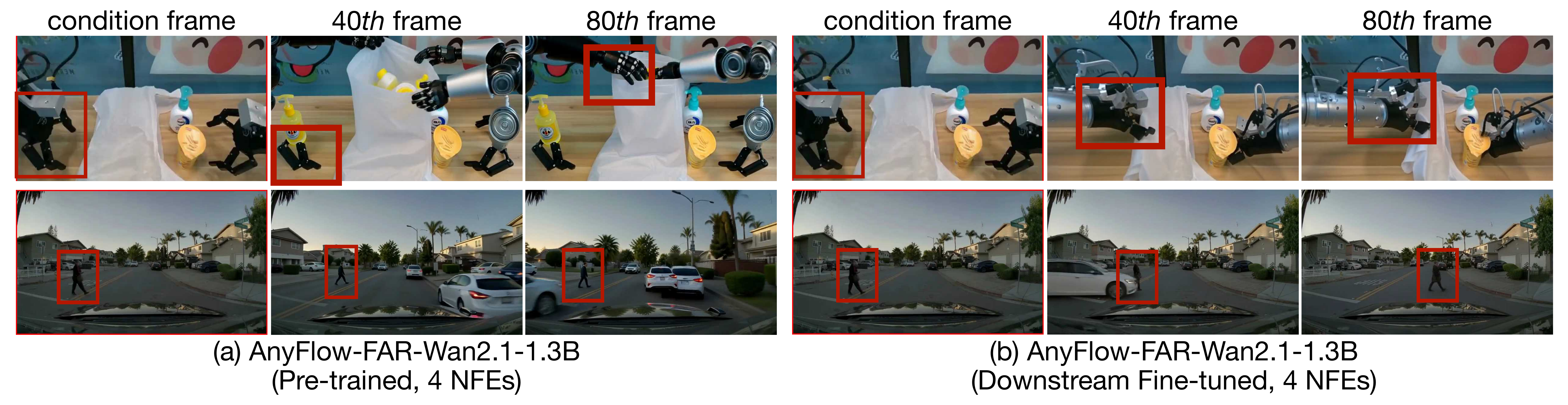
Figure 8 解读：下游可视化强调同一个 causal AnyFlow-FAR backbone 在 T2V/I2V/V2V 中都能保持多步可用；I2V 总分 87.87 只用 4 NFE，已接近或略高于 50×2 NFE 的 Wan2.1-I2V-14B。

5.4 消融与效率

Design	NFEs	Bidirectional Overall	Causal Overall
Flow Matching Training	$4\times 2$	74.64	76.80
Flow Matching Training	$32\times 2$	83.83	83.50
Consistency ODE-Init	4	80.44	73.97
Consistency ODE-Init	32	82.86	77.55
Flow Map Training	4	81.75	80.48
Flow Map Training	32	83.40	83.13
Consistency ODE-Init + Consistency Backward Simulation	4 / 32	82.96 / 79.80	82.49 / 79.64
Flow Map Training + Consistency Backward Simulation	4 / 32	83.55 / 82.96	82.99 / 83.49
Flow Map Training + Flow Map Backward Simulation	4 / 32	83.48 / 83.96	83.54 / 83.96

训练开销表显示：forward training 中 differential derivation 把 causal/bidirectional 成本推到 10.4/16.8 s/iter；on-policy 中 4-step Flow Map Backward Simulation 比 consistency simulation 贵 15.7%/22.5%，但在 16 steps 时成本仍为 53.1/51.2 s/iter，比 consistency 的 93.8/96.6 低 43.4%/47.0%。这支持作者的核心效率论点：shortcut simulation 对大 NFE 更划算。

5.5 Limitations and conclusions

局限：训练仍依赖强 teacher 和 teacher-generated video 数据；Stage 2 需要 real/fake teacher score，工程复杂度高；VBench/I2V 分数不能完全覆盖长视频时序一致性和用户偏好；released config 与 paper Stage-2 iteration 数存在 800 vs 1200 的差异，复现实验时应以目标 checkpoint 对应 config 为准。

核心 takeaway：AnyFlow 的创新点不是更复杂的 reward 或更强 teacher，而是把 distillation 的几何对象从 endpoint consistency 换成 flow map transition，并让 on-policy correction 也沿这个 transition space 反传。这个改动直接修复了少步蒸馏模型“多给步数不变好”的失败模式。

为什么有效：forward flow map training 提供可组合的 transition operator；flow map backward simulation 把 DMD 的 endpoint KL 梯度变成短链路可反传的 self-rollout correction；interpolated timestep conditioning 与 loss weighting 则让从 pretrained Wan2.1 迁移到 $(t,r)$ 双时间输入时不破坏原模型稳定性。

局限：训练仍依赖强 teacher 和 teacher-generated video 数据；Stage 2 需要 real/fake teacher score，工程复杂度高；VBench/I2V 分数不能完全覆盖长视频时序一致性和用户偏好；released config 与 paper Stage-2 iteration 数存在 800 vs 1200 的差异，复现实验时应以目标 checkpoint 对应 config 为准。

可复用点：若已有视频扩散 backbone 的少步蒸馏在大 NFE 退化，可以优先检查目标是否过度端点化；把 scheduler 改成显式 $t\to r$ transition，再用 on-policy self-rollout 做 DMD/RL-like correction，可能比继续调 consistency loss 更直接。