Beyond Language Modeling: An Exploration of Multimodal Pretraining

Authors: Shengbang Tong*, David Fan*, John Nguyen*, Ellis Brown, Gaoyue Zhou, Shengyi Qian, Boyang Zheng, Theophane Vallaeys, Junlin Han, Rob Fergus, Naila Murray, Marjan Ghazvininejad, Mike Lewis, Nicolas Ballas, Amir Bar, Michael Rabbat, Jakob Verbeek, Luke Zettlemoyer, Koustuv Sinha, Yann LeCun, Saining Xie Affiliations: FAIR, Meta, New York University arXiv: 2603.03276 Project Page: beyond-llms.github.io

1. Motivation (研究动机)

当前基础模型的发展主要由语言预训练驱动，但文本本质上是对现实世界的有损压缩。高质量文本数据有限且趋于枯竭，而视觉世界提供了无穷的信号流，捕捉了语言遗漏的物理规律、几何关系和因果性。

现有的多模态预训练研究存在以下核心问题:

• 设计空间不透明: 原生多模态模型的设计空间（视觉表示、数据混合、架构选择）缺乏系统研究
• 混杂变量: 大多数方法从预训练语言模型初始化，无法分离统一训练本身带来的能力与从语言预训练继承的能力
• 模态竞争假设未验证: 业界普遍假设视觉与语言在同一模型中会相互干扰，但缺乏从零开始的受控实验验证

本文的核心目标是通过从零开始的受控预训练实验，系统研究统一多模态预训练的关键设计维度，隔离各变量的影响，为构建真正的统一多模态模型提供实证指导。

---

2. Idea (核心思想)

本文采用 Transfusion 框架（语言用 next-token prediction，视觉用 diffusion/flow matching），在文本、视频、图文对、动作条件视频上从零训练单一模型，系统研究五个核心维度并得出四个关键建议:

1. S1 - 统一视觉表示: Representation Autoencoder (RAE) 提供最优的统一视觉表示，在理解和生成上均优于 VAE，无需双编码器架构
2. S2 - 拥抱多样数据: 视觉数据不会降低语言性能，多模态联合训练产生跨模态协同效应
3. S3 - 解锁世界建模: 统一多模态预训练自然涌现世界建模能力，仅需 1% 领域数据即可饱和
4. S4 - 使用 MoE: Mixture-of-Experts 高效扩展多模态训练，自然学习模态特定专家化，缩小视觉-语言 scaling 不对称性

---

3. Method (方法)

3.1 整体框架

Figure 1 解读: 整体架构为单一 decoder-only Transformer，接收文本（通过 Text Tokenizer）和视觉（通过冻结的 Vision Encoder）两种输入。文本分支使用 next-token prediction，视觉分支使用 flow matching 进行 next visual state prediction。底部五个模块对应论文研究的五个维度: Visual Representation、Data、World Model、Architecture、Scaling Behavior。

3.2 训练与推理机制

语言建模损失

对文本序列 $(x_1,\dots ,x_n)$，最小化标准自回归交叉熵:

$${\mathcal{L}}_{\text{LM}}=-\sum _{i=1}^n\log p_{\theta }(x_i\mid x_{<i})$$

Flow Matching 损失

令 $z_0$ 为图像/视频帧的 clean latent，$ϵ\sim \mathcal{N}(0,I)$。采样 $t\sim \mathcal{U}[0,1]$，构造插值 latent $z_t=(1-t)ϵ+t{z}_0$。模型预测速度场 $v_{\theta }(z_t,t,\text{context})$，最小化:

$${\mathcal{L}}_{\text{flow}}={\mathbb{E}}_{t,z_0,ϵ}\left[\Vert v_{\theta }(z_t,t,\cdot )-(z_0-ϵ){\Vert }_2^2\right]$$

混合训练目标

每个 batch 混合多种数据源（纯文本、视频、图文对、动作条件数据），优化加权目标:

$$\mathcal{L}={\lambda }_{\text{LM}}{\mathcal{L}}_{\text{LM}}+{\lambda }_{\text{flow}}{\mathcal{L}}_{\text{flow}}$$

默认 ${\lambda }_{\text{LM}}=1.0$，${\lambda }_{\text{flow}}=3.0$。

因果视觉与语言 Masking

使用 FlexAttention 实现混合 masking 策略:

• 文本: 标准因果 mask，只关注前序 token
• 视觉: Block-wise 因果 mask，同一帧内 token 双向 attend，但只能因果关注前序帧/文本

推理 (Modal-Switching)

def modal_switching_inference(model, prompt_tokens):
    """Modal-switching inference: 动态切换文本生成与视觉去噪"""
    output = []
    for step in autoregressive_loop(model, prompt_tokens):
        token = model.sample_next_token(context=output)
        if token == "<BOI>":
            # 切换到视觉生成模式
            noise = sample_gaussian(shape=(256,))  # 16x16 grid
            z_t = noise
            for t in euler_steps(num_steps=25):
                v = model.predict_velocity(z_t, t, context=output)
                z_t = z_t + v * dt
            image_latent = z_t
            pixels = decoder.decode(image_latent)
            output.append("<BOI>")
            output.append(image_latent)
            output.append("<EOI>")
        else:
            output.append(token)
    return output

3.3 模型与 Tokenization

Figure 2 解读: 展示四种训练数据类型的示例。Text: 纯网络文本; Image+Text: 图文配对（MetaCLIP/Shutterstock）; Action: 动作条件导航视频（含 dx, dy, dyaw, rel_t 数值动作）; Video: 纯视频帧序列。

Backbone: Decoder-only Transformer，从零训练，与 Transfusion 类似但使用简单线性投影层替代 U-Net。默认模型 2.3B 总参数，1.5B 激活参数（因 modality-specific FFN）。

文本 Token: LLaMA-3 BPE tokenizer，记为 $\text{T}$。

视觉 Token: 冻结视觉编码器将图像映射为 latent token，记为 $\text{I}$。所有帧预处理为 224x224。每帧产生 256 个 token（16x16 grid）。

Modality-Specific FFN: 每个 self-attention block 内使用两个独立 FFN（文本一个、视觉一个），替代共享 FFN。

Figure 3 解读: Radar 图对比 Modality-Specific FFN 与 Shared FFN 在七个指标上的表现。Modality-Specific FFN（蓝色）在所有指标上均优于或持平 Shared FFN（灰色），特别是在 DPGBench、GenEval 和 Avg VQA 上有明显提升，同时降低了 text perplexity。

3.4 视觉表示选择 (RAE vs VAE vs Raw Pixels)

Figure 4 解读: 对比不同视觉编码器在五个指标上的表现。SigLIP 2（RAE 类语义编码器）在 DPGBench、GenEval、Avg VQA 上均取得最佳成绩，同时保持与纯文本 baseline 可比的 text perplexity。SD-VAE 和 FLUX.1 VAE 在生成和理解上均不如语义编码器。Raw Pixel 在 VQA 上也有竞争力，但生成质量差距明显。

研究了三族编码器:

• VAE: SD-VAE (Stable Diffusion), FLUX.1 VAE — 低维 latent，传统生成首选
• RAE (Representation Autoencoder): SigLIP 2 So400m, DINOv2-L, WebSSL-L — 高维语义 latent
• Raw Pixels: 直接将 RGB 值 patchify 为 14x14 patch

核心发现: 语义编码器（特别是 SigLIP 2）在理解和生成上均优于 VAE，颠覆了”理解用语义编码器、生成用 VAE”的双编码器范式。

def encode_visual_tokens(image, encoder_type="siglip2"):
    """视觉 token 编码流程"""
    image = resize(image, (224, 224))
 
    if encoder_type in ["siglip2", "dinov2", "webssl"]:
        # RAE: 语义编码器, 直接 14x14 patch -> 256 tokens
        latent = frozen_encoder(image)  # shape: (256, d_encoder)
        tokens = linear_proj_in(latent)  # shape: (256, d_model)
    elif encoder_type in ["sd_vae", "flux_vae"]:
        # VAE: 8x8 patch -> 32x32 = 1024 latent patches
        latent = vae_encoder(image)  # shape: (1024, d_latent)
        # PixelUnshuffle(2): 32x32 -> 16x16, channel x4
        latent = pixel_unshuffle(latent, factor=2)  # shape: (256, d_latent*4)
        tokens = linear_proj_in(latent)  # shape: (256, d_model)
    elif encoder_type == "raw_pixel":
        # Raw: 14x14 RGB patches -> 256 tokens
        patches = patchify(image, patch_size=14)  # shape: (256, 14*14*3)
        tokens = linear_proj_in(patches)
    return tokens

3.5 数据组合与协同效应

Figure 5 解读: 对比不同数据组合对 text perplexity 的影响。Text + Video 在 DCLM 上匹配甚至优于纯文本 baseline，说明视频数据与语言建模兼容。加入 MetaCLIP 后 PPL 略有上升，因为图文 caption 的文本分布与预训练文本不同。

Figure 6 解读: I/T 数据对视觉能力至关重要。Text + Video 不含 I/T 数据，因此无法生成图像。加入 MetaCLIP 后解锁图像生成和理解能力，全数据混合在 VQA 上表现最佳。

Image-Text 分布分析:

数据源	MetaCLIP	MetaCLIP (Recap)	SSTK
Cosine Distance (与 DCLM)	0.196	0.286	0.215

策略: 用 MetaCLIP 做 image-to-text (I2T), SSTK 做 text-to-image (T2I)，各取所长。

跨模态协同效应:

Figure 8 解读: 左图显示在固定视觉 token 预算下，增加文本 token 持续改善 diffusion loss 和 GenEval 分数，超越纯视觉 baseline。右图显示用 20B VQA token + 80B 异构数据（视频/MetaCLIP/文本）训练，所有混合变体均超越 100B 纯 VQA baseline，证明多样预训练优于专项数据扩增。

3.6 世界建模 (Navigation World Model)

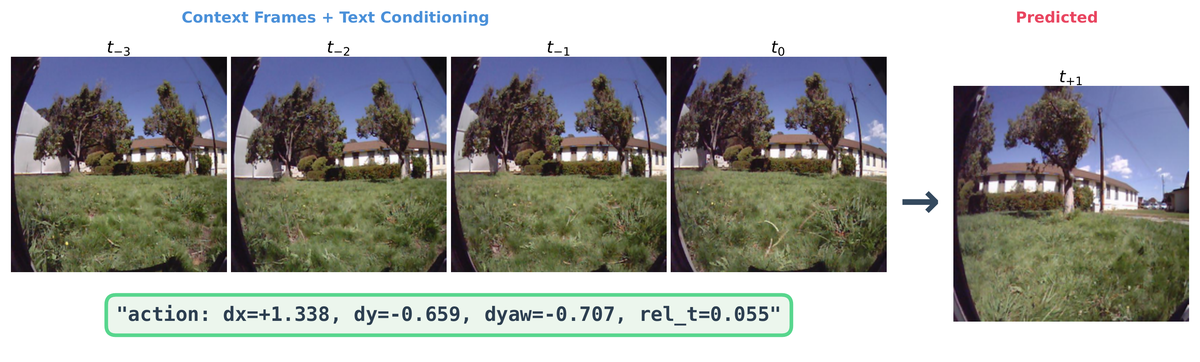
Figure 11 解读: 导航世界建模任务示意。输入 4 个上下文帧 + 文本格式的导航动作（如 “action: dx=+1.338, dy=-0.659, dyaw=-0.707, rel_t=0.055”），模型预测下一个视觉状态。关键创新: 动作直接编码为文本 token，无需专用 adapter。

任务格式化为 $\text{I}+\text{T}\to \text{I}$ (给定上下文帧 + 文本动作 → 预测目标帧):

def format_nwm_sequence(context_frames, action, target_frame):
    """将导航世界建模任务格式化为统一序列"""
    sequence = []
    for frame in context_frames:  # 4 context frames
        tokens = encode_visual_tokens(frame)
        sequence.extend(["<BOI>", tokens, "<EOI>"])
 
    # 动作编码为自然语言文本 token
    action_text = f"action: dx={action.dx:.3f}, dy={action.dy:.3f}, "
    action_text += f"dyaw={action.dyaw:.3f}, rel_t={action.rel_t:.3f}"
    sequence.extend(tokenize(action_text))
 
    # 目标帧 (训练时提供, 推理时生成)
    target_tokens = encode_visual_tokens(target_frame)
    sequence.extend(["<BOI>", target_tokens, "<EOI>"])
    return sequence

世界建模能力从通用预训练涌现:

Figure 13 解读: 左右两图分别显示 ATE 和 RPE 随 NWM 数据比例的变化。性能在仅 1% 领域数据时即饱和，说明世界建模的核心能力来自通用多模态预训练，而非领域专属数据。

3.7 MoE 架构设计

Expert Granularity

定义 expert granularity $G$:

$$G=\frac{4d_{\text{model}}}{d_{\text{expert}}}$$

$G=1$ 对应 16 个大 expert ($d=8192$, Top-1 routing)，$G=64$ 对应 1024 个小 expert ($d=128$, Top-64 routing)。

Figure 15 解读: 四组图展示 Granularity $G$ 从 1 增至 64 的影响。更高 granularity（到 $G=16$）显著改善所有指标。视觉在 $G=4$ 饱和，语言在 $G=16$ 饱和。对 RAE (SigLIP 2) $x$-pred 优于 $v$-pred；对 VAE (FLUX.1) $v$-pred 更好。

Sparsity Scaling

Figure 16 解读: 固定 16 个 active expert，增加 total expert 数从 32 到 1008（active ratio 从 50% 降至 1.6%），text PPL 和 diffusion loss 持续下降，GenEval 持续上升。证明 MoE 的稀疏扩展在多模态 setting 中同样有效。

Per-Modality Shared Expert

三种 expert 配置对比:

Configuration	DCLM PPL $\downarrow$	Notes PPL $\downarrow$	Diff. Loss $\downarrow$	GenEval $\uparrow$
No Shared Expert	14.802	27.392	0.484	0.360
Global Shared Expert	14.794	27.249	0.483	0.364
Per-Modality Shared Expert	14.785	27.161	0.483	0.367

Per-Modality Shared Expert 效果最佳: 为文本和视觉各指定 1 个 always-active shared expert，加上 Top-15 routed expert。

class MoELayer:
    """Mixture-of-Experts layer with per-modality shared experts"""
    def __init__(self, d_model, d_expert, num_experts, num_active, num_shared_per_modality):
        self.num_experts = num_experts          # e.g., 256
        self.num_active = num_active            # e.g., 16
        self.num_shared = num_shared_per_modality  # e.g., 1 per modality
 
        # Expert pool
        self.experts = [FFN(d_model, d_expert) for _ in range(num_experts)]
        # Per-modality shared experts (always active)
        self.text_shared = FFN(d_model, d_expert)
        self.vision_shared = FFN(d_model, d_expert)
        # Router
        self.router = Linear(d_model, num_experts)
 
    def forward(self, x, modality):
        # Router scores
        scores = softmax(self.router(x))  # (batch, num_experts)
        # Select top-(k-1) routed experts (reserve 1 slot for shared)
        top_indices = topk(scores, k=self.num_active - self.num_shared)
 
        # Compute routed expert outputs
        output = weighted_sum([self.experts[i](x) for i in top_indices],
                              weights=scores[top_indices])
 
        # Add modality-specific shared expert
        if modality == "text":
            output += self.text_shared(x)
        else:
            output += self.vision_shared(x)
        return output

涌现的模态特化

Figure 18 解读: 每层 256 个 expert 按路由偏好分类为 Text Expert ($S_i>0.5$)、Vision Expert ($S_i<-0.5$) 和 Multimodal Expert。早期层以 text expert 为主，后期层逐渐增加 vision 和 multimodal expert。模型自然学习了”先分别处理、后融合”的策略。

Figure 20 解读: 四层（Layer 0/5/10/15）的 expert selection rate 散点图，x 轴为图像生成时的选择率，y 轴为图像理解时的选择率。所有层 Pearson 相关 $r\ge 0.90$，说明视觉理解和生成共享相同的 expert，模型自然收敛到统一的视觉表示。

3.8 设计选择叠加验证

Figure 21 解读: 从 Transfusion baseline 出发，逐步叠加最佳设计选择。每一步同时改善 Perplexity 和 DPG score: Shared FFN → Mod.-Specific FFN (PPL 15.93→15.13, DPG 0.45→0.47); SD-VAE → SigLIP 2 (PPL→15.06, DPG→0.57); Dense → MoE (PPL→12.49, DPG→0.63); $v$-pred → $x$-pred (DPG→0.65)。最终模型: Modality-specific FFN + SigLIP 2 + MoE + $x$-pred。

3.9 代码-论文映射表

Paper Concept	Source File	Key Class/Function
代码搜索未找到开源实现	—	—

---

4. Experimental Setup (实验设置)

训练配置

参数	值
Backbone	Decoder-only Transformer, 16 layers, $d_{\text{model}}=2048$
Attention	GQA, 32 query heads, 8 KV heads
FFN Multiplier	1.5x
默认模型参数	2.3B total (modality-specific FFN), 1.5B active
MoE 配置	$G=16$, $d_{\text{expert}}=512$, Top-16 active, 256 total experts
MoE 大模型参数	13.5B total, 1.5B active
序列长度	4096
Batch Size	128 GPUs x 4 per GPU = 512 sequences (~2M tokens/step)
优化器	AdamW, peak LR $3\times 10^{-4}$, 1000 warmup steps, cosine decay to 5%
训练规模	520B text + 520B multimodal tokens (约1T总tokens)
硬件	64-128 NVIDIA H200 GPUs (8 nodes)
视觉编码器	SigLIP 2 So400m (frozen)
文本 Tokenizer	LLaMA-3 BPE
视觉 Token 数	256 per image/frame (16x16 grid)
图像分辨率	224x224
CFG Scale	3.0 (inference)
Euler Steps	25 (inference)
条件 Dropout	10% (训练时, 用于 CFG)
损失权重	${\lambda }_{\text{LM}}=1.0$, ${\lambda }_{\text{flow}}=3.0$

数据源

数据类型	模态	来源
Text	$\text{T}\to \text{T}$	DCLM
Video	$\text{I}\to \text{I}$	YouTube-Temporal 1B, SomethingSomething V2, Kinetics
Image-Text Pairs	$\text{I}\to \text{T},\text{T}\to \text{I}$	MetaCLIP, in-house Shutterstock
Action-Conditioned	$\text{I}+\text{T}\to \text{I}$	NWM, in-house Text-Annotated Videos

评估指标

• 文本: DCLM PPL, Notes PPL (OOD)
• 视觉生成: DPGBench, GenEval, COCO FID, Diffusion Loss
• 视觉理解: 16 个 Cambrian VQA benchmarks 平均准确率 (MMBench, Seed, GQA, AI2D, MathVista, MMMU 等)
• 世界建模: ATE (Absolute Trajectory Error), RPE (Relative Pose Error)
• 知识生成: WISE benchmark

---

5. Experimental Results (实验结果)

5.1 视觉表示 (Section 3)

• SigLIP 2 (RAE) 在 DPGBench、GenEval、VQA 上同时取得最佳分数
• 所有视觉表示的 text PPL 与纯文本 baseline 相近，raw pixel 甚至略优
• 语义编码器在生成质量（DPGBench, GenEval）上一致优于 VAE 编码器
• Multimodal 预训练后微调 VQA: SigLIP 2 达到 40.3%（vs text-only 预训练的 33.9%）

5.2 数据组合 (Section 4)

• Text + Video 在 DCLM PPL 上匹配纯文本 baseline（约 13.3 vs 13.3）
• MetaCLIP 引入 caption 分布偏移导致 PPL 略升（~0.5 point）
• 策略性使用不同 I/T 源（MetaCLIP 用于 I2T + SSTK 用于 T2I）优于单一来源
• 20B VQA + 80B 异构数据 (37.9%) > 100B 纯 VQA (35.7%)

5.3 世界建模 (Section 5)

• 多模态预训练 (+ Video 50B): ATE 1.410, RPE 0.414 — 优于 NWM-only 100B (ATE 1.669, RPE 0.450)
• 性能在 1% NWM 数据时饱和（ATE ~1.2, RPE ~0.38）
• 模型可零样本接受自然语言导航指令（如 “get out of the shadow!“）

5.4 MoE 架构 (Section 6)

• Granularity $G=16$ 为最优: DCLM PPL 从 ~20 (G=1) 降至 ~14.5
• Sparsity scaling: 从 32 experts 到 1008 experts (1.5B → 51.5B 总参数, active 恒为 ~1.5B), PPL 和 GenEval 持续改善
• Per-Modality Shared Expert 在所有指标上最优
• Vision expert 不按 diffusion timestep 特化 (CV scores ~0.15)，理解与生成共享 expert ($r\ge 0.90$)

5.5 设计选择叠加 (Section 6.3)

最终最优配置从 Transfusion baseline 逐步提升:

配置	Perplexity $\downarrow$	DPG Score $\uparrow$
Transfusion (baseline)	15.93	0.45
+ Mod.-Specific FFN	15.13	0.47
+ SigLIP 2	15.06	0.57
+ MoE	12.49	0.63
+ $x$-pred	12.69	0.65

5.6 Scaling Laws (Section 7)

Dense 模型的 IsoFLOP 分析发现模态 scaling 不对称:

• Language: $N_{\text{opt}}\propto C^{0.47}$, $D_{\text{opt}}\propto C^{0.53}$ — 接近 Chinchilla 平衡
• Vision: $N_{\text{opt}}\propto C^{0.37}$, $D_{\text{opt}}\propto C^{0.63}$ — 视觉更 data-hungry

视觉所需数据相对于语言随模型规模增长: $D_{\text{opt}}\propto N^{0.57}$，在 1B 参数时需 14x，1T 参数时需 51x。

MoE 模型缩小了这一差距:

• Language: $a\approx 0.41$, $b\approx 0.59$
• Vision: $a\approx 0.36$, $b\approx 0.64$
• 参数 scaling 指数差距从 0.10 (dense) 缩小到 0.05 (MoE)

Figure 23 解读: Dense 模型的 IsoFLOP 曲线。上排为 Language，下排为 Vision。左列为 IsoFLOP 曲线（不同 compute budget 下 loss vs 参数量），中间两列分别为最优参数 $N_{\text{opt}}$ 和最优 token 数 $D_{\text{opt}}$ 随 FLOPs 的 power law 拟合，右列对比两模态。Vision 的 $N_{\text{opt}}$ 曲线斜率（0.37）明显低于 Language（0.47），说明视觉需要更多数据而非更大模型。

Figure 25 解读: MoE 模型的 IsoFLOP 曲线。与 dense 模型相比，MoE 将 vision-language 的参数 scaling 指数差距从 0.10 缩小到 0.05。右列对比图中两模态的 $N_{\text{opt}}$ 曲线更为接近，说明 MoE 的稀疏性有效调和了模态间 scaling 的不对称性。

5.7 知识感知生成 (WISE Benchmark)

Figure 22 解读: WISE benchmark 评估知识感知图像生成能力。MoE + SigLIP 2 在所有六个知识类别（Biology, Chemistry, Cultural, Physics, Space, Time）上取得最高分。语义编码器 + MoE 组合优于 VAE-based 模型 3-4 倍。

5.8 Compute Efficiency

Figure 24 解读: Dense Multimodal 模型与 Text-Only 和 T2I-Only baseline 的 scaling 对比。在全计算范围内，Dense Multimodal 在四个指标上均匹配或超越 unimodal baselines。在 $10^{21}$ FLOPs 时: Notes PPL 23.7 vs 23.8, DCLM PPL 13.3 vs 13.6, DPG 0.622 vs 0.598, FID 39.3 vs 41.5。

Figure 26 解读: MoE Multimodal 与 unimodal MoE baselines 对比。统一模型在四个指标上紧密跟踪对应的 unimodal counterpart。在 $10^{21}$ FLOPs 时: DCLM PPL 12.3 vs 12.0 (Text-Only), FID 39.2 vs 39.8 (T2I-Only)。MoE 使单一模型匹配两个领域的专用模型性能。