Streaming Autoregressive Video Generation via Diagonal Distillation

Authors: Jinxiu Liu, Xuanming Liu, Kangfu Mei, Yandong Wen, Ming-Hsuan Yang, Weiyang Liu Affiliations: South China University of Technology, Westlake University, Johns Hopkins University, UC Merced, CUHK Venue: ICLR 2026

机构: South China University of Technology, Westlake University, Johns Hopkins University, UC Merced, CUHK

链接: arXiv:2603.09488 | GitHub: Sphere-AI-Lab/diagdistill

关键词: Diffusion Distillation, Autoregressive Video Generation, Streaming, Flow Distribution Matching, KV Cache

---

1. Motivation (研究动机)

核心问题

现有 diffusion-based 视频生成模型在实时流式生成方面存在重大限制:

1. 双向注意力的局限: 主流视频扩散模型 (如 Wan2.1) 使用 bidirectional attention 同时去噪所有帧, 要求未来帧可用, 无法用于实时流式场景 (游戏模拟、机器人学习等)
2. 自回归扩散模型的推理瓶颈: 虽然 AR 扩散模型天然适合流式生成, 但每个 chunk 仍需多步去噪, 导致延迟高
3. 现有蒸馏方法的缺陷: 图像蒸馏方法 (如 DMD) 直接用于视频效果差, 因为:
   • 忽略时间维度的上下文信息
   • 减少步数后运动连贯性下降
   • 长序列生成时误差累积导致过饱和 (oversaturation)

关键观察

隐式噪声级别预测 (Exposure Bias):

Figure 2 解读: 当训练数据使用显式噪声帧作为条件 (如 Causvid), 下一个 chunk 的预测本质上是在做隐式的”下一步噪声级别预测”。图中展示了即使使用单步预测, 随着 chunk 推进图像也逐渐变清晰。这说明后续 chunk 可以利用前面已充分去噪的 chunk 作为结构先验, 从而使用更少的去噪步骤。这一观察直接启发了”前多后少”的非对称去噪策略。

---

2. Idea (核心思想)

核心思想: Diagonal Distillation

提出一种 flow-aware 对角蒸馏框架, 同时在时间维度 (chunk 间) 和去噪步数维度上利用信息, 包含三个核心创新:

1. Diagonal Denoising (对角去噪): 非对称步数分配 — 前面的 chunk 用更多去噪步, 后面的 chunk 逐步减少到 2 步
2. Diagonal Forcing (对角强制训练): 在训练时显式模拟对角去噪轨迹, 通过受控噪声注入弥合训练-推理分布差距
3. Flow Distribution Matching (光流分布匹配): 将显式时序建模引入蒸馏 loss, 确保运动一致性

与现有方法的关系

方法	训练策略	问题
Teacher Forcing	条件为 clean ground-truth 帧	训练-推理不一致, 长序列误差累积
Diffusion Forcing	条件为 noisy latents	去噪基于噪声上下文, 但推理时用 clean 上下文
Self Forcing	条件为模型自身预测	早期低质量预测影响学习
Diagonal Forcing (Ours)	混合 clean + model-generated, 对角排列	兼顾鲁棒性和质量

Figure 10 解读: 四种时序训练策略的对比可视化。(a) Teacher Forcing: 绿框表示 ground-truth 帧; (b) Diffusion Forcing: 红框表示 noisy latents; (c) Self Forcing: 红框表示模型自身预测; (d) Diagonal Forcing (本文): 绿框和红框按对角线混合排列。Diagonal Forcing 的核心创新在于: 对于当前目标帧, 最近的帧来自模型自身预测 (红), 更早的帧来自 ground-truth (绿), 这种对角模式精确模拟了 Diagonal Denoising 的推理场景, 从而对齐训练和推理分布。

---

3. Method (方法)

3.1 Overall Framework

Figure 3 解读: Diagonal Denoising 的完整流程示意。从 Chunk 1 到 Chunk 7, 去噪步数从 5 步逐渐减少到 2 步 (步数配置 = [5, 4, 3, 2, 2, 2, 2])。关键细节: (1) 前 3 个 chunk 使用不同步数的蒸馏模型; (2) 从 Chunk 4 开始固定使用 2-step 蒸馏模型; (3) 每个 chunk 的倒数第二步输出被加噪后作为 KV cache 传递给下一个 chunk (黄色虚线框); (4) 这种设计使后续 chunk 可以继承前面 chunk 丰富的外观信息。

3.2 Preliminary: Distribution Matching Distillation (DMD)

Score Function:

$$s_{\text{real}}(x_t,t)={\nabla }_{x_t}\log p_{\text{real},t}(x_t)=-\frac{x_t-{\alpha }_t{\mu }_{\text{real}}(x_t,t)}{{\sigma }_t^2}(1)$$

DMD Loss Gradient:

$$\nabla {\mathcal{L}}_{\text{DMD}}={\mathbb{E}}_t\left({\nabla }_{\theta }\text{KL}(p_{\text{fake},t}\Vert p_{\text{real},t})\right)=-{\mathbb{E}}_t\left(\int \left(s_{\text{real}}(F(G_{\theta }(z),t),t)-s_{\text{fake}}(F(G_{\theta }(z),t),t)\right)\frac{d{G}_{\theta }(z)}{d\theta }dz\right)(2)$$

Regression Loss:

$${\mathcal{L}}_{\text{reg}}=E_{(z,y)}d(G_{\theta }(z),y)(3)$$

3.3 Diagonal Denoising: Progressive Step Reduction

前 3 个 chunk ($k=1,2,3$) 使用递减步数 ($s_k=5,4,3$):

$${\mathbf{X}}_k={\mathcal{D}}_{s_k}({\mathbf{Z}}_k|{\tilde{\mathbf{X}}}_{<k})(4)$$

其中 ${\mathbf{Z}}_k\sim \mathcal{N}(0,\mathbf{I})$ 是高斯噪声, ${\tilde{\mathbf{X}}}_{<k}$ 是之前已加噪的 chunk。

Chunk $k\ge 4$ 使用固定 2-step 去噪:

$${\mathbf{C}}_k=\mathcal{T}({\tilde{\mathbf{X}}}_{k-1}),{\mathbf{X}}_k={\mathcal{D}}_2({\mathbf{Z}}_k|{\mathbf{C}}_k|{\mathbf{C}}_k)(5)$$

def diagonal_denoising(M: int, step_schedule: list, models: dict) -> list:
    """Diagonal Denoising with Noisy KV Cache (Algorithm 1)
    Args:
        M: number of chunks
        step_schedule: e.g. [5, 4, 3, 2, 2, 2, 2]
        models: distilled models {s: Theta_s, 2: Theta_2}
    """
    outputs = []      # output buffer
    kv_cache = []      # cached KV states
 
    for k in range(1, M + 1):
        eps = sample_gaussian()  # eps ~ N(0, I)
 
        if k <= 4:  # Base Phase: progressive step reduction
            x_k = sample_gaussian()  # X_k^(0) ~ N(0, I)
            s_k = step_schedule[k - 1]
            for t in range(1, s_k + 1):
                x_k = denoise_step(x_k, outputs[:k-1], kv_cache, models[s_k])
                if t == s_k - 1:  # penultimate step: cache noisy result
                    cache_noisy_result(x_k, kv_cache)
            x_tilde_k = mix(x_k, eps)
 
        else:  # Extension Phase: fixed 2-step generation
            c_k = compute_condition(outputs[k - 2])  # condition from previous chunk
            x_step1 = denoise_step(sample_gaussian(), c_k, kv_cache, models[2])
            cache_noisy_result(x_step1, kv_cache)  # cache after step 1
            x_step2 = denoise_step(x_step1, c_k, kv_cache, models[2])
            x_tilde_k = mix(x_step2, eps)
 
        outputs.append(x_tilde_k)
 
    return outputs
 
def cache_noisy_result(x, kv_cache: list, alpha_k: float):
    """Add noise to intermediate result and cache its KV representation."""
    eps = sample_gaussian()
    x_interim = sqrt(alpha_k) * x + sqrt(1 - alpha_k) * eps
    kv_cache.append(compute_kv(x_interim))

3.4 Diagonal Forcing: Contextual Prior Propagation

训练时通过受控噪声注入模拟对角去噪轨迹:

$${\tilde{\mathbf{X}}}_{k-1}=\sqrt{{\alpha }_{k-1}}\cdot {\mathbf{X}}_{k-1}+\sqrt{1-{\alpha }_{k-1}}\cdot ϵ,ϵ\sim \mathcal{N}(0,\mathbf{I})(6)$$

其中 ${\alpha }_{k-1}$ 控制对角路径上的噪声 schedule。这显式维护了去噪轨迹: ${\mathbf{X}}_k\to {\tilde{\mathbf{X}}}_{k-1}\to {\mathbf{X}}_{k-1}$, 其中 ${\tilde{\mathbf{X}}}_{k-1}$ 作为 chunk $k$ 的 KV cache 输入。

def diagonal_forcing_training(chunks_gt: list, alpha_schedule: list, t_noise: int = 100):
    """Diagonal Forcing Training: simulate diagonal denoising trajectory during training."""
    for iteration in training_iterations:
        for k in range(1, len(chunks_gt)):
            # Step 1: Add controlled noise to previous chunk's clean output
            eps = sample_gaussian()  # eps ~ N(0, I)
            alpha_prev = alpha_schedule[t_noise]  # alpha_{k-1} at timestep=100
            x_tilde_prev = sqrt(alpha_prev) * chunks_gt[k-1] + sqrt(1 - alpha_prev) * eps
 
            # Step 2: Use noisy result as KV cache condition
            kv_cache = compute_kv(x_tilde_prev)
 
            # Step 3: Standard DMD training on current chunk
            z = sample_gaussian()
            x_pred = generator(z, text_cond, kv_cache)
 
            # Step 4: Combined loss (spatial DMD + regression + flow matching)
            loss = L_DMD(x_pred) + L_reg(x_pred) + gamma * (L_flow_DMD(x_pred) + L_flow_reg(x_pred))
            loss.backward()

3.5 Flow Distribution Matching

运动分布散度度量:

$${\mathcal{E}}_{\text{motion}}=D_{\text{KL}}\left(p_{\text{teacher}}(\mathcal{F}(\mathbf{x})|{\mathbf{x}}_t)\Vert p_{\text{student}}(\mathcal{F}(\mathbf{x})|{\mathbf{x}}_t)\right)(7)$$

Flow DMD Loss Gradient:

$${\nabla }_{\varphi }{\mathcal{L}}_{\text{DMD}}^{\text{flow}}\triangleq {\mathbb{E}}_t\left({\nabla }_{\varphi }\text{KL}(p_{\text{gen,flow},t}\Vert p_{\text{data,flow},t})\right)(8)$$ $${\nabla }_{\varphi }{\mathcal{L}}_{\text{DMD}}^{\text{flow}}\approx -{\mathbb{E}}_t\left[\int \left(s_{\text{data}}^{\text{flow}}(\Psi (G_{\varphi }(ϵ),t),t)-s_{\text{gen},\xi }^{\text{flow}}(\Psi (G_{\varphi }(ϵ),t),t)\right)\frac{d{G}_{\varphi }(ϵ)}{d\varphi }dϵ\right](9)$$

Flow Score Function:

$$s^{\text{flow}}({\mathbf{x}}_t,t)={\nabla }_{{\mathbf{x}}_t}\log p(\mathcal{F}(\mathbf{x})|{\mathbf{x}}_t)(10)$$

Flow Regression Loss:

$${\mathcal{L}}_{\text{reg}}^{\text{flow}}={\mathbb{E}}_{t,ϵ}\left[\Vert \mathcal{F}(G_{\varphi }^{\text{teacher}}(ϵ,t))-\mathcal{F}(G_{\varphi }^{\text{student}}(ϵ,t)){\Vert }_2^2\right](11)$$

运动特征提取器 $\mathcal{F}(\cdot )$ 的实现: 轻量级 Conv-MLP, 直接在 latent space 操作:

1. 计算连续 latent 帧之间的差值 (latent difference)
2. 通过 2 层卷积提取局部运动模式
3. MLP 进行特征自适应
4. Student 通过梯度反传更新, Teacher 通过 EMA 更新

class MotionFeatureExtractor:
    """Flow Distribution Matching: lightweight Conv-MLP on latent space."""
    def __init__(self):
        self.conv_layers = Conv2d(...)  # 2 convolutional layers
        self.mlp = MLP(...)            # feature adaptation
 
    def forward(self, latent_sequence):
        # latent_sequence: [B, F, C, H, W]
        # Step 1: Frame-wise difference (temporal motion signal)
        diff = latent_sequence[:, 1:] - latent_sequence[:, :-1]  # [B, F-1, C, H, W]
        # Step 2: Convolutional motion extraction
        motion_features = self.conv_layers(diff)
        # Step 3: MLP adaptation
        return self.mlp(motion_features)
 
def flow_distribution_matching_step(G_student, G_teacher, F_student, F_teacher, eps, t: float):
    """One training step of Flow Distribution Matching."""
    # Extract motion features from student and teacher generators
    flow_student = F_student(G_student(eps, t))
    flow_teacher = F_teacher(G_teacher(eps, t))
 
    # Flow DMD gradient: score difference (analogous to spatial DMD)
    flow_dmd_loss = compute_score_diff(s_data_flow=flow_teacher, s_gen_flow=flow_student)
    # Flow regression loss
    flow_reg_loss = (flow_teacher - flow_student).pow(2).mean()
 
    return flow_dmd_loss, flow_reg_loss
 
# Training setup
F_student = MotionFeatureExtractor()       # updated via gradient descent
F_teacher = EMA(F_student, momentum=0.99)  # updated via EMA: theta^- <- mu*theta^- + (1-mu)*theta

3.6 Total Loss

$${\mathcal{L}}_{\text{Total}}={\lambda }_{\text{spatial}}{\mathcal{L}}_{\text{DMD}}+{\mathcal{L}}_{\text{reg}}+\gamma \left({\lambda }_{\text{flow}}{\mathcal{L}}_{\text{DMD}}^{\text{flow}}+{\mathcal{L}}_{\text{reg}}^{\text{flow}}\right)(12)$$

其中 ${\lambda }_{\text{spatial}}=4$, ${\lambda }_{\text{flow}}=4$, $\gamma =1.0$ (flow loss weight)。

---

4. Experimental Setup (实验设置)

训练配置

配置项	值
Base Model	Wan2.1-T2V-1.3B (Flow Matching)
初始化模型	LongLive-1.3B (long-context video)
分辨率	832 x 480
帧率	16 FPS
Chunk Size	3 帧
KV Cache Window	4 chunks (12 帧)
Denoising Steps	[1000, 100] (warped timesteps)
Timestep Shift	$k=5.0$
Learning Rate	2e-6 (generator), 4e-7 (critic)
Optimizer	Adam (${\beta }_1=0$, ${\beta }_2=0.999$)
EMA Weight	0.99, start at step 200
Training Iterations	600
训练时间	< 2h (64 H100), < 16h (8 H100 w/ grad accum)
Mixed Precision	BF16
FSDP Strategy	Hybrid Full Sharding
Gradient Checkpointing	Enabled
Noise Schedule	Flow Matching ($t^{\prime }=\frac{k\cdot t/1000}{1+(k-1)(t/1000)}\times 1000$, $k=5$)
Diagonal Forcing Timestep	100 (最优, 见 ablation)
Prompts	VidProM filtered + LLM-extended

推理配置

配置项	值
GPU	Single NVIDIA H100
VAE	Tiny VAE (9.84M params, 10x faster decoding)
Step Schedule (5s video)	[4, 3, 2, 2, 2, 2, 2] → 总 NFEs = 34
KV Cache Memory	17.5 GB
Latent Overlap	9 帧
torch.compile	可选 (进一步加速)

评估指标

使用 VBench 评估框架:

• Temporal Quality: Subject Consistency, Background Consistency, Temporal Flickering, Motion Smoothness, Dynamic Degree 的均值
• Frame Quality: Aesthetic Quality, Imaging Quality 的均值
• Text Alignment: Object Class, Multiple Objects, Human Action, Color, Spatial Relationship, Scene, Appearance, Style, Temporal Style 的均值

---

5. Experimental Results (实验结果)

5.1 Main Comparison (Table 1)

Model	Throughput (FPS)	First-Frame Latency (s)	Speedup	Total Score	Quality	Semantic
Wan2.1	0.78	103	1.0x	84.26	85.30	80.09
SkyReels-V2	0.49	112	0.91x	82.67	84.70	74.53
MAGI-1	0.19	282	0.36x	79.18	82.04	67.74
Causvid	17.0	0.69	149.3x	81.20	84.05	69.80
Self-Forcing	17.0	0.69	149.3x	84.31	85.07	81.28
DiagDistill (Ours)	31.0	0.37	277.3x	84.48	85.26	81.73

关键数据:

• 相比 Wan2.1 baseline 实现 277.3x 加速, 5 秒视频生成仅需 2.61 秒 (31 FPS)
• 相比之前最快的 Self-Forcing, 延迟降低 1.53x (0.37s vs 0.69s)
• 保持与 full-step model 接近的视觉质量 (85.26 vs 85.30)

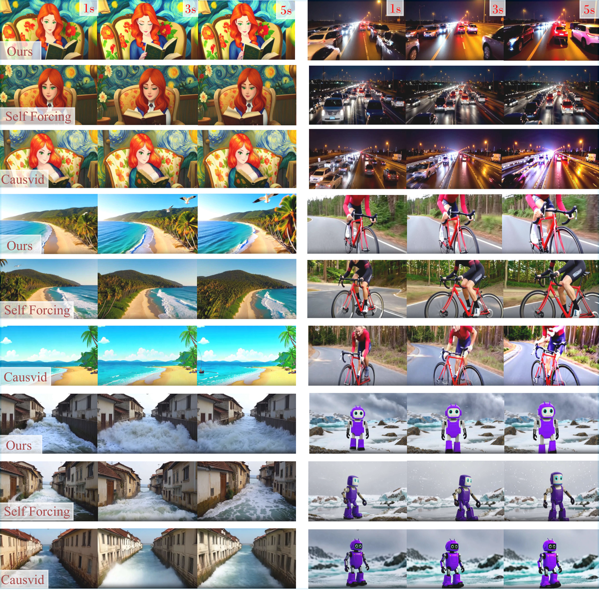
Figure 4 解读: 三种方法的视觉质量对比。每组 3 行分别展示 Ours / Self Forcing / Causvid 的结果。可以观察到: (1) 本文方法在复杂运动和纹理场景中表现更好, 帧过渡更平滑; (2) Causvid 在长序列中出现明显的饱和度失真和动态伪影; (3) Self-Forcing 在部分场景中出现模糊和变形。

Figure 1 解读: Diagonal Distillation 与 Causvid、Self-Forcing 的主要对比。左侧展示三种方法的速度差异, 右侧展示 5 秒视频在 1s/3s/5s 时刻的帧质量。DiagDistill 仅需 2.61 秒完成生成, 比 Causvid 和 Self-Forcing (4.91 秒) 快 1.88 倍, 同时保持可比的视觉质量。

5.2 Ablation Studies

Key Components (Table 2):

Ablation Variant	Temporal Quality	Frame Quality	Text Alignment	Total Score
Without Diagonal Forcing	92.1	60.1	26.9	83.58
Without Flow Loss	92.5	60.8	27.8	84.18
Without Diagonal Denoising	95.1	63.2	28.6	84.46
Full Method (Ours)	94.9	63.4	28.9	84.48

Figure 5 解读: 两个关键超参数的 ablation 分析。(a) Diagonal Forcing 的噪声注入 timestep: timestep=100 在所有指标上达到最优, 太大 (1000) 导致结构先验模糊、运动幅度下降, 太小 (0) 等价于使用 clean 帧导致过饱和; (b) Flow loss weight: weight=1.0 在时序质量、帧质量和文本对齐之间达到最佳平衡, 过大的 flow 约束反而有害。

Figure 6 解读: Flow Distribution Matching 的运动效果对比。(a) 无 motion loss: 物体运动幅度极小, 几乎是静止的; (b) 有 motion loss: 整个画面运动幅度显著增大。这验证了 Flow Distribution Matching 在保持少步去噪下运动动态性方面的关键作用。

Denoising Configurations (Table 3):

Steps Config	Temporal	Frame	Text	NFEs	Latency (s)	Throughput (FPS)
5333333	95.0	63.9	29.1	46	0.34	22.5
4322222	94.9	63.4	28.9	34	0.23	31.0
4222222	93.4	62.3	27.8	32	0.23	32.0
5432222	94.8	63.1	29.0	40	0.23	29.7

最终选择 4322222 配置: 仅 34 NFEs, 质量接近最优 (5333333), 但延迟和吞吐量显著更优。

5.3 Long Video Generation

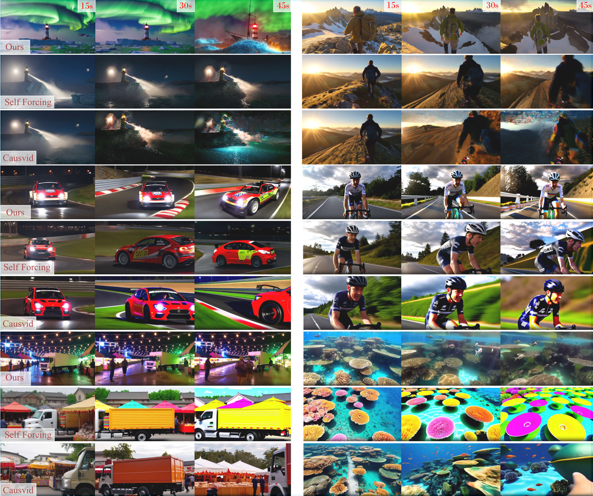
Figure 7 解读: 45 秒长视频生成的定性对比。每组 3 行: Ours / Self-Forcing / Causvid。可以明显看到其他方法在长序列中出现饱和度失真和质量衰减, 而本文方法在整个 45 秒内保持细节和一致性。

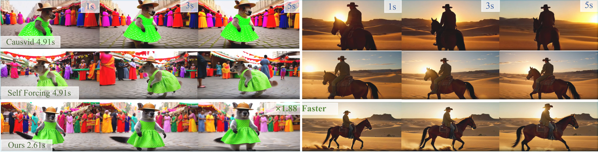
Figure 8 解读: 长视频生成的定量评估。左图: 用户偏好率 — DiagDistill 在与所有 baseline 的对比中均获得多数偏好 (vs Causvid 66.1%, vs Wan2.1 62.7%, vs SkyReels-V2 57.9%, vs MAGI-1 54.2%, vs Self-Forcing 59.3%)。右图: 随时间推移的平均质量 — 本文方法在 45 秒内保持稳定的高质量 (>50%), 而其他方法质量随时间明显下降。

5.4 Dynamic Prompting

Figure 9 解读: 动态 prompting 的长视频生成示例。该功能允许用户在时间轴的任意点引入新的文本描述, 创建包含场景变换和动作演变的复杂叙事。图中展示了四个不同的动态 prompting 视频: 人物行走穿越不同场景、打扫房间、海边电话亭随时间变化、以及赛博朋克摩托车追逐。

5.5 Acceleration Analysis (Appendix E)

四大加速源:

1. 去噪步数减少: 从 uniform 多步 → 前多后少, 总 NFEs 从 ~48 降至 34
2. 高效 KV Cache: 直接在 noisy latent 上做 KV caching (不需额外 clean frame 计算), 消除冗余计算
3. 优化注意力窗口: KV cache 窗口从 Self-Forcing 的 6 chunks 减至 4 chunks, 显存从 19.2GB 降至 17.5GB
4. Tiny VAE: 解码参数从 73.3M 降至 9.84M, 解码时间从 1.67s 降至 0.12s (10x+)

---

Code-to-Paper Mapping

Paper 概念	代码位置	说明
DMD Loss (Eq. 2)	model/dmd.py: _compute_kl_grad()	计算 real/fake score 差值作为 KL gradient, 包含 spatial 和 motion gradient
Regression Loss (Eq. 3)	model/dmd.py: compute_distribution_matching_loss()	在 DMD loss 之外还计算 x0 prediction regression
Diagonal Denoising (Eq. 4-5)	pipeline/causal_inference.py: inference()	use_diagonal_denoising flag 控制步数递减, block_index 决定 step schedule
Diagonal Forcing (Eq. 6)	pipeline/streaming_training.py	use_dia_forcing flag, 加噪 timestep 由 context_noise 控制
Flow Distribution Matching (Eq. 7-11)	model/dmd.py: _compute_kl_grad()	grad_motion 计算帧间差分的 score 差异
Flow Regression (Eq. 11)	Motion feature extractor in training	Conv-MLP on latent diff, EMA teacher-student
Total Loss (Eq. 12)	trainer/distillation.py	组合 spatial DMD + reg + flow DMD + flow reg
Noisy KV Cache (Algorithm 1)	pipeline/causal_inference.py	CacheNoisyResult: 对中间结果加噪后缓存 KV
Step Schedule [4,3,2,2,2,2,2]	configs/diadistill_inference.yaml	denoising_step_list + use_diagonal_denoising
Tiny VAE	taehv.py + inference.py: TinyVAEWrapper	包装 TAEHV 进行快速解码
Streaming Training	model/streaming_training.py: StreamingTrainingModel	管理流式生成状态、KV cache 复用、chunk-wise loss
Training Config	configs/diadistill_train_init.yaml	lr=2e-6, batch=1, 21 frames, local_attn=12