Radial Attention: O(n log n) Sparse Attention with Energy Decay for Long Video Generation

Authors: Xingyang Li*, Muyang Li*, Tianle Cai, Haocheng Xi, Shuo Yang, Yujun Lin, Lvmin Zhang, Songlin Yang, Jinbo Hu, Kelly Peng, Maneesh Agrawala, Ion Stoica, Kurt Keutzer Affiliations: MIT, NVIDIA, Princeton, UC Berkeley, Stanford, First Intelligence Venue: NeurIPS 2025

1. Motivation (研究动机)

核心问题

视频 Diffusion Model 的核心瓶颈在于 3D dense attention 的 O(n^2) 计算复杂度。随着视频帧数增加，token 数量线性增长（例如 HunyuanVideo 生成 5 秒 720p 视频需要约 110K tokens），attention 计算量呈二次方增长，使得长视频的训练和推理代价极高。

现有方法的不足

1. SVG (Sparse VideoGen)：动态地将每个 attention head 分类为 spatial 或 temporal，分别施加对应的 sparse mask。但存在两个问题：(a) runtime profiling 在未见过的视频长度上不可靠；(b) 无法加速训练，只能加速推理；(c) 忽略了 temporal decay，对远帧分配了不必要的计算。
2. Linear Attention (SANA 等)：用线性复杂度替代 softmax attention，但需要大幅修改模型架构，且往往难以捕捉局部细节，导致质量下降。
3. STA (Sliding Tile Attention)：固定 3D sliding window 提供局部注意力，但限制了 long-range dependency。
4. PowerAttention：虽然也是 O(n log n)，但忽略视频数据固有的时空结构，效果不佳。

物理直觉

自然界中信号和波随距离传播时会损失能量。作者在 video diffusion model 的 post-softmax attention score 中发现了类似的现象：attention score 随 token 间的时空距离增大而指数衰减。作者称此现象为 Spatiotemporal Energy Decay。这一发现直接启发了 Radial Attention 的设计——将 energy decay 转化为 compute density decay。

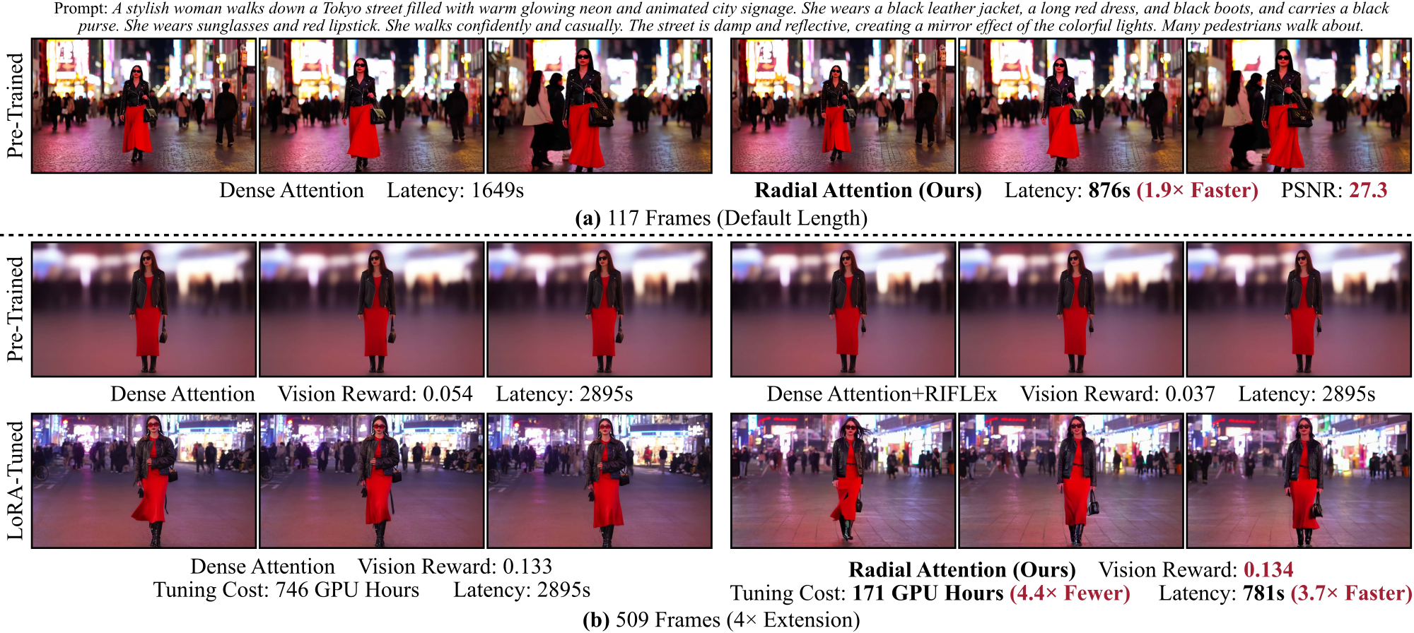
Figure 1 解读：Figure 1 展示了 Radial Attention 的核心效果。上半部分 (a) 是 pre-trained HunyuanVideo 在默认 117 帧长度下的对比：Dense Attention 需要 1649s，Radial Attention 仅需 876s（1.9x 加速），PSNR 达到 27.3，视觉质量几乎无损。下半部分 (b) 是 4x 长度扩展（509 帧）场景：Dense Attention + Full fine-tuning 需要 746 GPU hours 训练和 2895s 推理；Radial Attention + LoRA 仅需 171 GPU hours（4.4x 节省）和 781s 推理（3.7x 加速），且 Vision Reward 更高（0.134 vs 0.133）。

---

2. Idea (核心思想)

核心洞察

Radial Attention 的核心思想可以用一句话概括：attention score 随时空距离指数衰减，因此计算密度也应该随时空距离指数衰减。

具体而言，作者将 energy decay 建模为指数函数：对于 frame i 中位置 k0 的 query token，frame j 中位置 l 的 key token 的 attention score 满足上界：

$$p_{js+l}\le C_{\text{rel}}{e}^{-\alpha |j-i_0|-\beta |l-k_0|}{p}_{i_{0}s+k_0}$$

其中 alpha 控制 temporal decay，beta 控制 spatial decay。这意味着：

• Temporal 维度：距离当前帧越远的帧，attention score 越低，可以分配更少的计算
• Spatial 维度：同一帧内距离越远的 token，attention score 越低，可以用更窄的 diagonal window

与 SVG 的统一

SVG 将 attention head 二分为 spatial head 和 temporal head，分别施加不同的 sparse mask。Radial Attention 用一个统一的 static mask 同时建模 spatial 和 temporal 的 sparsity：

• 中心 band（band 0，即相同帧或相邻帧）保留完整的 spatial interaction，相当于 SVG 的 spatial attention
• 外层 band 逐步减少 spatial window width 和 temporal sampling frequency，实现 temporal decay

设计优势

1. Static mask：无需 runtime profiling，可同时加速训练和推理
2. O(n log n) 复杂度：介于 O(n^2) dense 和 O(n) linear 之间的最佳平衡
3. 保留 softmax attention：不修改底层 attention 机制，只剪枝不重要的 token pair，因此可以用 LoRA 轻量微调扩展到更长视频
4. Block-friendly：以 128x128 block 为粒度计算，适配现代 GPU 硬件

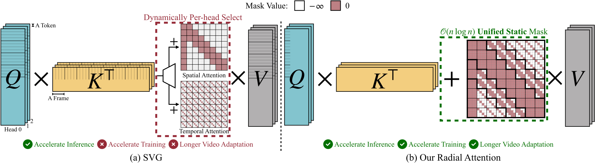
Figure 2 解读：对比 SVG 和 Radial Attention 的 pipeline。左侧 (a) SVG 需要为每个 head 动态选择 spatial 或 temporal mask，每个 head 只能是其中一种；右侧 (b) Radial Attention 使用一个统一的 static mask，所有 head 共享，同时包含 spatial 和 temporal 信息。关键区别在于：SVG 只能加速推理，不能加速训练，也不支持更长视频适配；Radial Attention 三者皆可。

---

3. Method (方法)

3.1 Spatiotemporal Energy Decay 的观测

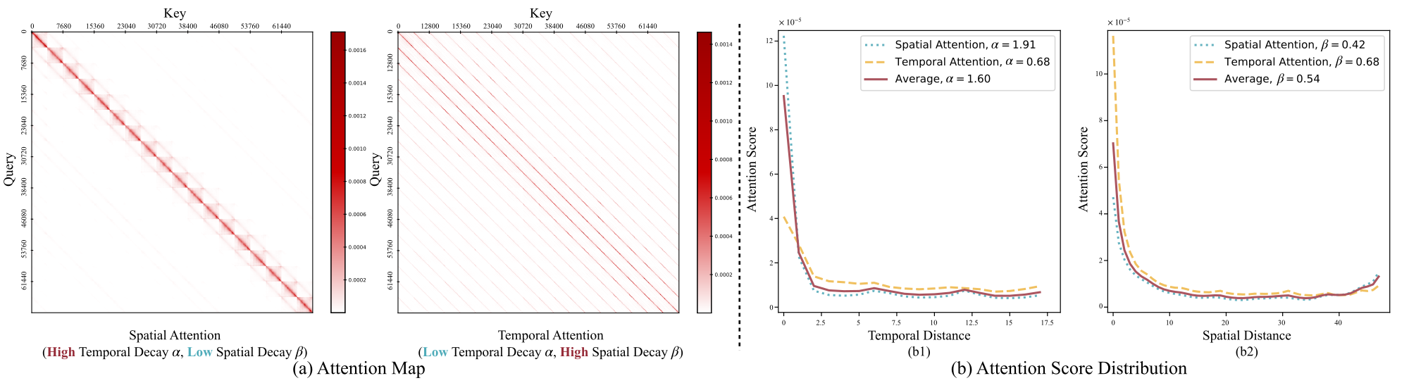
Figure 3 解读：(a) 展示了 HunyuanVideo 的两种 post-softmax attention map：左侧是 spatial attention（高 temporal decay alpha，低 spatial decay beta），每个 token 主要关注相邻帧的邻近位置；右侧是 temporal attention（低 temporal decay，高 spatial decay），每个 token 主要关注跨帧的相同空间位置。(b) 定量展示了 decay 分布：(b1) 随 temporal distance 增大，相同空间位置的平均 attention score 下降；(b2) 随 spatial distance 增大，同帧内的平均 attention score 下降。红色虚线为指数函数拟合，R^2 > 0.985，验证了指数衰减假设。

3.2 Radial Attention Mask 构建

Radial Attention mask 的构建包含两个维度的 decay：

Temporal Density Decay

沿时间维度，frame i 到 frame j 之间的计算密度为：

$$\text{density}(i,j)={\left(\frac{1}{2}\right)}^{\lfloor {\log }_2(\max (|i-j|,1))\rfloor }$$

这形成了 2*ceil(log2(max(f,2))) - 1 个 band 的结构，以主对角线（band 0）为中心。Band 0 保持 100% 计算密度，每向外一层 band 宽度翻倍但密度减半。

Spatial Density Decay

在每个 frame-to-frame attention block 内部，attention 集中在空间位置相似的 token 上，形成对角线结构。随着帧间距离增大，对角线的宽度缩小：

$$\text{diagonal\_width}(i,j)=\lfloor \frac{s}{2^{\lfloor {\log }_2\max (|i-j|,1)\rfloor }}\rfloor$$

当宽度小于 1 时，不再缩窄对角线，而是降低对角线的采样频率。

形式化定义

4D attention mask $\tilde{M}\in \{-\infty ,0{\}}^{f\times f\times s\times s}$ 的构建规则：

$${\tilde{M}}_{i,j,k,l}=\{\begin{array}{ll}0,& \text{if }{2}^{\lfloor {\log }_2\max (|i-j|,1)\rfloor }\le s\text{ and }|k-l|+1\le \frac{s}{2^{\lfloor {\log }_2\max (|i-j|,1)\rfloor }}\\ 0,& \text{if }|i-j|\mathrm{mod}\lceil \frac{2^{\lfloor {\log }_2\max (|i-j|,1)\rfloor }}{s}\rceil =0\text{ and }k=l\\ -\infty ,& \text{otherwise}\end{array}$$

此外还加入 attention sink（第一帧保持全连接）以提升质量。

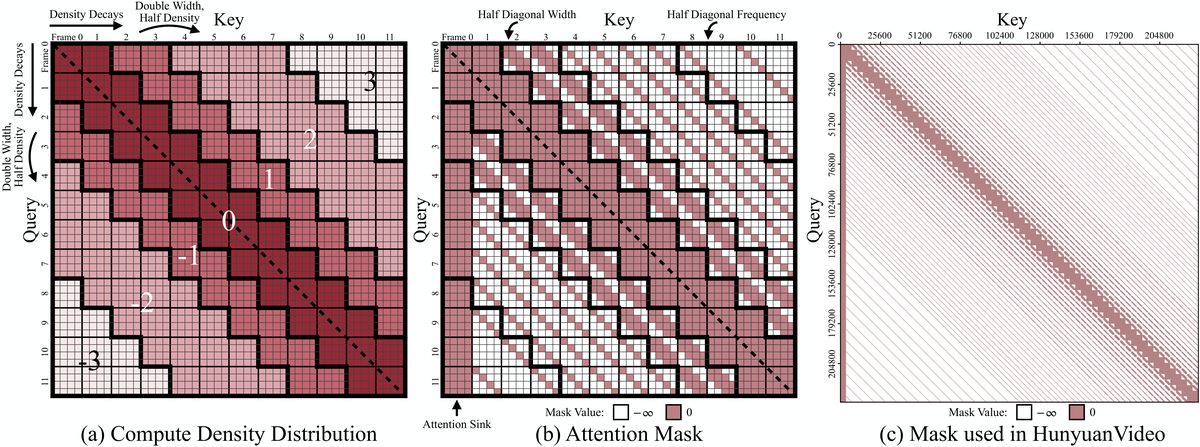
Figure 4 解读：(a) Compute Density 分布图：以 12 帧为例，中心 band 保持 100% 密度（最深红色），向外每层 band 宽度翻倍、密度减半（颜色逐渐变浅），形成”辐射状”衰减——这正是 Radial Attention 名称的由来。(b) 对应的 Attention Mask：白色为 0（允许 attend），红色为 -inf（masked）。可以看到中心 band 的 frame-to-frame block 有宽对角线，外层 band 对角线变窄且采样变稀疏。底部有 attention sink。(c) 实际在 HunyuanVideo 上使用的 253 帧 720p 视频的完整 mask，展示了大规模场景下 mask 的稀疏性。

3.3 复杂度分析

Mask 中零元素（允许计算的 token pair）数量的上界为：

$$\text{\#zeros}\le 4s^{2}f{\log }_{2}f=4sn({\log }_{2}n-{\log }_{2}s)$$

对于长视频（f 很大，s 固定），复杂度为 O(n log n)，其中 n = f * s。

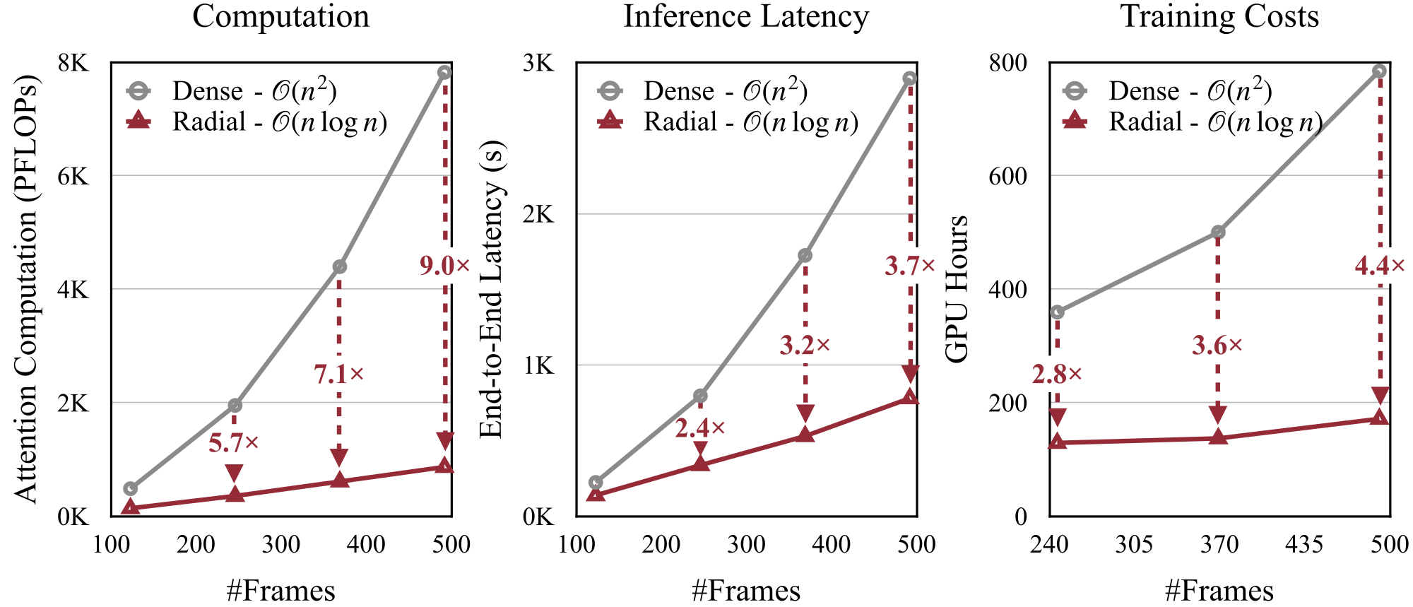
Figure 5 解读：三组图分别展示 Computation（PFLOPs）、Inference Latency（秒）、Training Costs（GPU hours）随帧数的增长趋势。Dense attention 为 O(n^2)（红色），Radial Attention 为 O(n log n)（蓝色）。在 509 帧 720p 视频上，Radial Attention 将 attention 计算量减少 9x，推理加速 3.7x，训练成本节省 4.4x。

3.4 Error Analysis

近似误差的 L1 bound 为：

$$\Vert \tilde{p}-p{\Vert }_1\le C_{\text{rel}}\left[\frac{8e^{-\beta (\frac{s}{2}+1)}}{(1-e^{-\alpha })(1-e^{-\beta })}+4\frac{1+e^{-\beta }}{1-e^{-\beta }}\frac{e^{-\alpha (s+1)}}{1-e^{-\alpha }}\right]=O(C_{\text{rel}}{e}^{-\min (\beta /2,\alpha )s})$$

误差随 alpha 和 beta 的增大指数衰减。实验中 Radial Attention 的 attention output MSE 为 3.9e-3，低于 SVG 的 4.4e-3 和 STA 的 1.5e-2。

3.5 LoRA-based Long Video Adaptation

Radial Attention 保留了 softmax attention 的基本结构，因此 pre-trained weights 大部分可以复用。通过在 Q, K, V, O projection 上加 LoRA adapter 进行轻量微调，即可适配更长视频。经验上 LoRA fine-tuning + Radial Attention 的效果甚至优于 full fine-tuning + dense attention。

Pseudocode

Radial Attention Mask 生成

def gen_radial_mask(num_frames, tokens_per_frame, block_size=128):
    """生成 Radial Attention 的 block-sparse mask"""
    n_blocks = (num_frames * tokens_per_frame) // block_size
    mask = zeros(n_blocks, n_blocks, dtype=bool)
 
    for i in range(num_frames):
        for j in range(num_frames):
            dist = abs(i - j)
 
            # Attention sink: 第一帧保持全连接
            if j == 0:
                local_mask = ones(tokens_per_frame, tokens_per_frame)
            else:
                # Temporal density decay: window width 随距离指数缩小
                group = bit_length(dist)  # = floor(log2(dist)) + 1
                window_width = tokens_per_frame // (2 ** group)
                window_width = max(window_width, block_size)
 
                # Spatial decay: 对角线 window
                local_mask = |col - row| <= window_width
 
                # 当 window_width < block_size 时，降低采样频率
                if window_width < block_size:
                    split_factor = block_size // window_width
                    if dist % split_factor != 0:
                        local_mask = zeros(...)  # 跳过此 frame pair
 
            # Shrink to block-level mask
            block_mask = shrink_to_blocks(local_mask, block_size)
 
            # 写入最终 mask
            mask[i_block_start:i_block_end, j_block_start:j_block_end] |= block_mask
 
    return mask

Radial Attention 推理

def radial_attention(Q, K, V, mask_map, block_size=128):
    """
    Q, K, V: [batch, seq_len, num_heads, head_dim]
    mask_map: 预计算的 MaskMap 对象
    """
    # Step 1: 获取 block-sparse mask（首次调用时生成并缓存）
    video_mask = mask_map.query_log_mask(Q, sparse_type="radial")
 
    # Step 2: 转换为 BSR (Block Sparse Row) 格式
    indptr = get_indptr_from_mask(video_mask, Q)   # [num_blocks + 1]
    indices = get_indices_from_mask(video_mask, Q)  # [nnz_blocks]
 
    # Step 3: 使用 FlashInfer BlockSparseAttention 执行
    bsr_wrapper = flashinfer.BlockSparseAttentionWrapper(workspace)
    bsr_wrapper.plan(indptr, indices, M, N, R=128, C=128, ...)
 
    # Video tokens: block-sparse attention
    output_video = bsr_wrapper.run(Q_video, K_video, V_video)
 
    # Text tokens: dense attention (text 部分 token 少，无需稀疏化)
    output_text = flashinfer.prefill(Q_text, K_all, V_all)
 
    return concat(output_video, output_text)

代码映射 (Code Mapping)

论文概念	代码文件	关键函数/类
Radial Attention mask 生成	radial_attn/attn_mask.py	gen_log_mask_shrinked()
Temporal density decay	radial_attn/attn_mask.py	get_window_width()
Spatial diagonal + frequency sampling	radial_attn/attn_mask.py	get_diagonal_split_mask()
Block-level mask 压缩	radial_attn/attn_mask.py	shrinkMaskStrict()
Mask 缓存管理	radial_attn/attn_mask.py	MaskMap class
FlashInfer BSR attention backend	radial_attn/attn_mask.py	FlashInferBackend()
SageAttention sparse backend	radial_attn/attn_mask.py	SpargeSageAttnBackend()
统一入口	radial_attn/attn_mask.py	RadialAttention()
HunyuanVideo 集成	radial_attn/models/hunyuan/	模型适配代码
Wan2.1 集成	radial_attn/models/wan/	模型适配代码

核心代码逻辑（attn_mask.py中的关键片段）：

get_window_width — 计算 frame i 到 frame j 的 spatial diagonal width：

def get_window_width(i, j, token_per_frame, sparse_type, num_frame, decay_factor=1, block_size=128, model_type=None):
    dist = abs(i - j)
    if dist <= 1:
        return token_per_frame  # 相邻帧保持全宽度
    group = dist.bit_length()   # floor(log2(dist)) + 1
    decay_length = 2 ** token_per_frame.bit_length() / 2 ** group * decay_factor
    return max(decay_length, block_size)  # 不低于 block_size

get_diagonal_split_mask — 当 window width 低于 block_size 时通过降低采样频率实现进一步稀疏化：

def get_diagonal_split_mask(i, j, token_per_frame, sparse_type, query):
    dist = abs(i - j)
    group = dist.bit_length()
    decay_length = 2 ** token_per_frame.bit_length() / 2 ** group
    if decay_length >= 128:  # threshold = block_size
        return ones(token_per_frame, token_per_frame)
    split_factor = int(128 / decay_length)
    if dist % split_factor == 0:
        return ones(...)  # 保留此 frame pair
    else:
        return zeros(...)  # 跳过此 frame pair

---

4. Experimental Setup (实验设置)

模型

Model	Parameters	Resolution	Default Length
Mochi 1	10B	480p	5s, 162 frames
HunyuanVideo	13B	720p (768x1280)	5s, 117/125 frames
Wan2.1-14B	14B	720p	5s, 69/81 frames

评估指标

• Vision Reward：近似人类评分（越高越好）
• PSNR / SSIM / LPIPS：与 original model output 的数值/感知相似度
• VBench-long：Subject Consistency, Aesthetic Quality, Image Quality

Baselines

• SVG（动态 spatial/temporal mask）
• STA（sliding tile attention，使用 FlashAttention-3）
• PowerAttention（power-of-two 距离 sparse attention）
• LongLoRA（shifted local attention）
• SANA（linear attention）
• RIFLEx（RoPE frequency 调整）
• Full fine-tuning with dense attention

实现细节

• 推理 backend: FlashInfer（BSR block-sparse attention）
• 训练 backend: FlashAttention-2
• Block size: 128 x 128
• 第一个 DiT block 保持 dense attention（质量考虑）
• 前 12 步 warmup 使用 dense attention
• 长视频微调：8x H100 GPU, OpenVid-1M 数据集中采样 2k 高质量视频
• 训练时间：HunyuanVideo 1621h, Mochi 817h, Wan2.1 15h

---

5. Experimental Results (实验结果)

5.1 Default Length Inference Acceleration (Table 1)

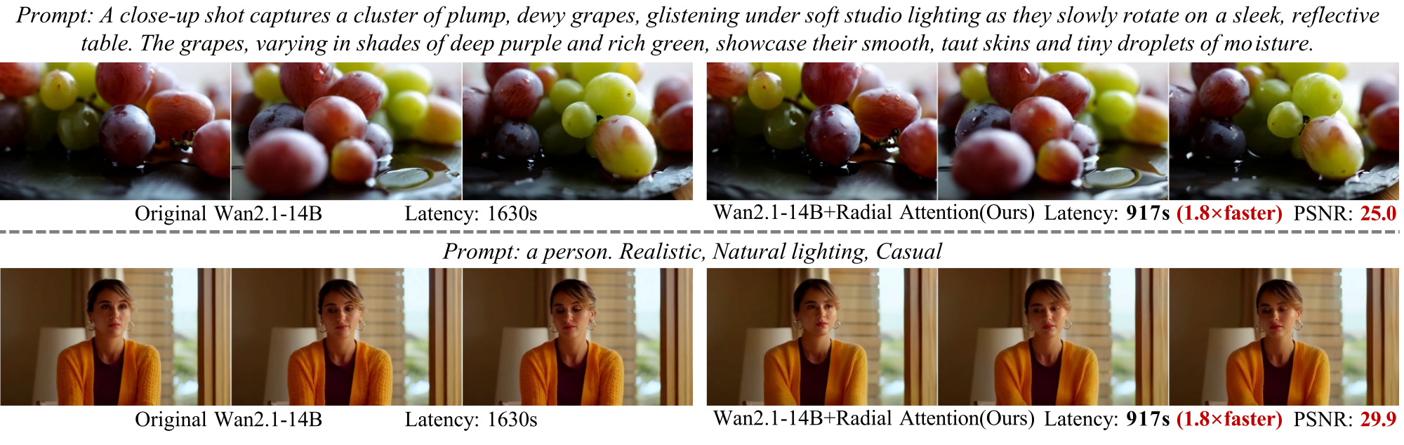
Figure 6 解读：Table 1 展示默认长度下的对比结果。Radial Attention 在相同计算预算下一致地在 PSNR、SSIM、LPIPS 上优于 STA 和 PA，同时匹配 SVG 的视觉保真度。在 HunyuanVideo 上实现 1.88x 加速（876s vs 1649s），在 Wan2.1 上实现 1.77x 加速（917s vs 1630s）。注意 STA 虽然速度稍快（2.29x），但使用了 FA3 而非 FA2，且视觉质量明显下降。

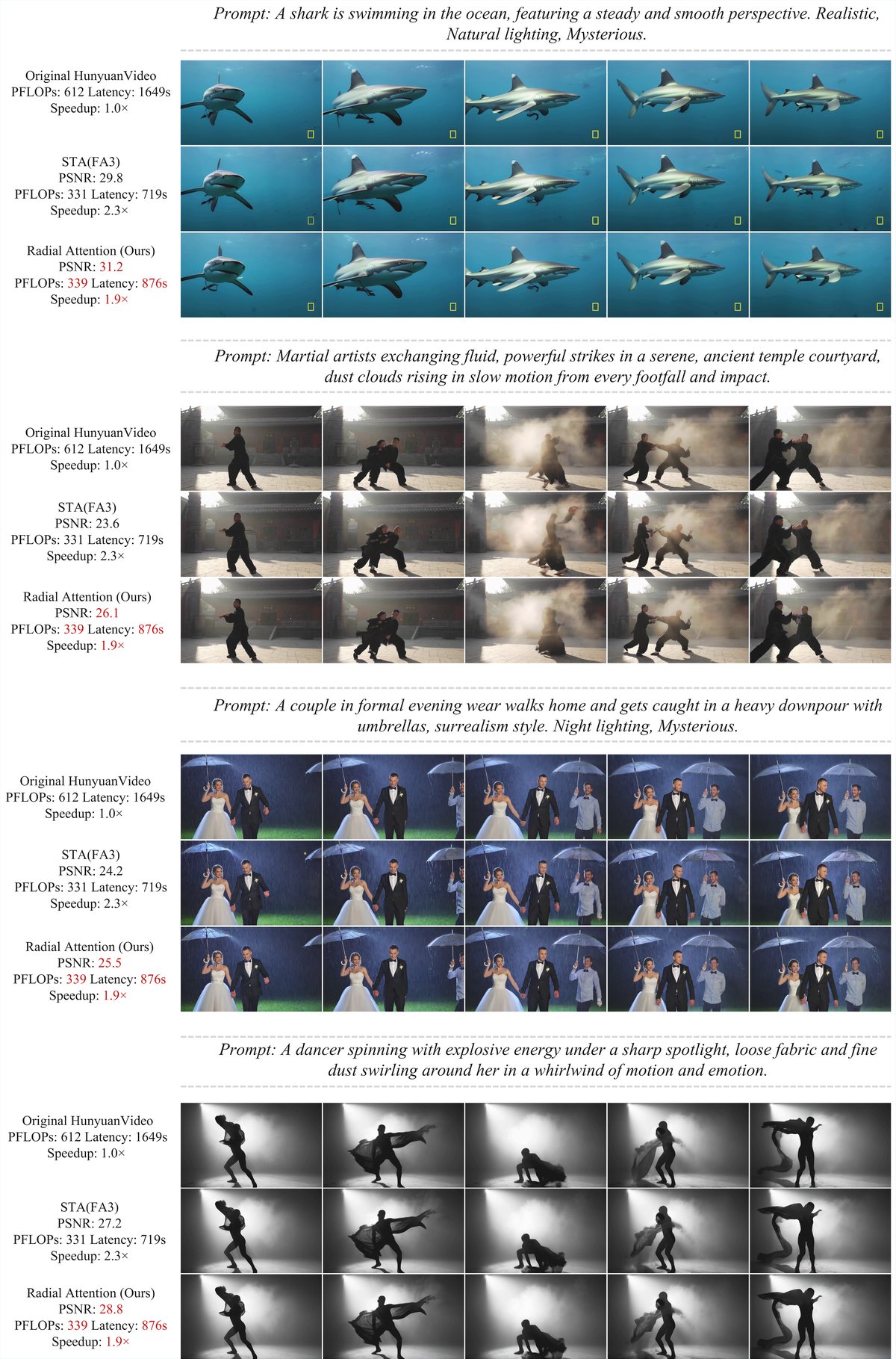
Figure 7 解读：HunyuanVideo 默认长度视觉对比。Radial Attention 在 HunyuanVideo 默认 117 帧上的生成结果与原始模型视觉质量几乎一致，PSNR 达到 27.3，同时延迟从 1649s 降至 876s（1.9x 加速）。

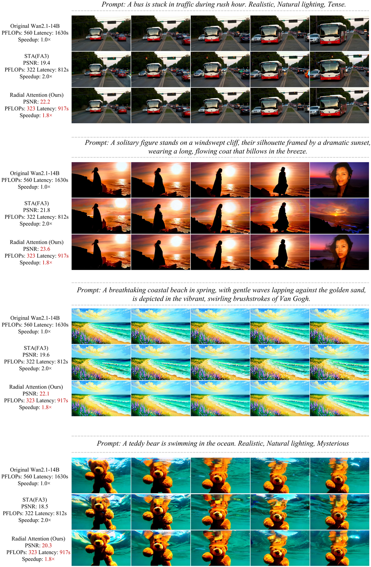
Figure 8 解读：Wan2.1-14B 默认长度视觉对比。Radial Attention 在 Wan2.1-14B 上同样保持了与原始模型高度一致的视觉质量，PSNR 达到 25.0，延迟从 1630s 降至 917s（1.8x 加速）。

Model	Method	PSNR	SSIM	LPIPS	Vision Reward	Speedup
HunyuanVideo	Original	-	-	-	0.141	-
	STA (FA3)	26.7	0.866	0.167	0.132	2.29x
	SVG	27.2	0.895	0.114	0.144	1.90x
	Ours	27.3	0.886	0.114	0.139	1.88x
Wan2.1-14B	Original	-	-	-	0.136	-
	STA (FA3)	22.9	0.830	0.171	0.132	2.01x
	SVG	23.2	0.825	0.202	0.114	1.71x
	Ours	23.9	0.842	0.163	0.128	1.77x

5.2 Long Video Generation (Table 2)

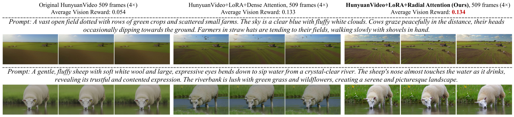
Figure 9 解读：HunyuanVideo 4x 长度扩展（509 帧）的视觉对比。左侧为原始 HunyuanVideo（0.054 Vision Reward），中间为 Dense Attention + LoRA（0.133），右侧为 Radial Attention + LoRA（0.134）。Radial Attention 的 LoRA 微调结果在视觉质量上与 dense attention 相当甚至更优，但训练成本低 4.4x，推理快 3.7x。

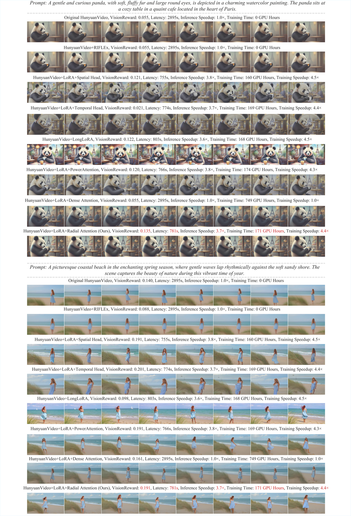
Figure 10 解读：HunyuanVideo 4x 扩展视觉对比。509 帧长视频生成效果。Radial Attention + LoRA 在视觉保真度和运动一致性上与 Dense Attention + LoRA 相当，但训练成本降低 4.4x，推理速度提升 3.7x。

关键结果（HunyuanVideo 4x = 509 帧）：

Method	Sparsity	Training Time (h)	Training Speedup	Inference Speedup	Vision Reward
Original	0.0%	-	-	1.0x	0.054
Full FT	0.0%	93.6	1.0x	1.0x	0.133
Ours	88.3%	16.2	2.78x	3.71x	0.134

Radial Attention 在 4x 长度扩展下达到 88.3% sparsity，推理加速 3.71x，训练加速 2.78x（成本节省 4.37x）。

5.3 Ablation Study

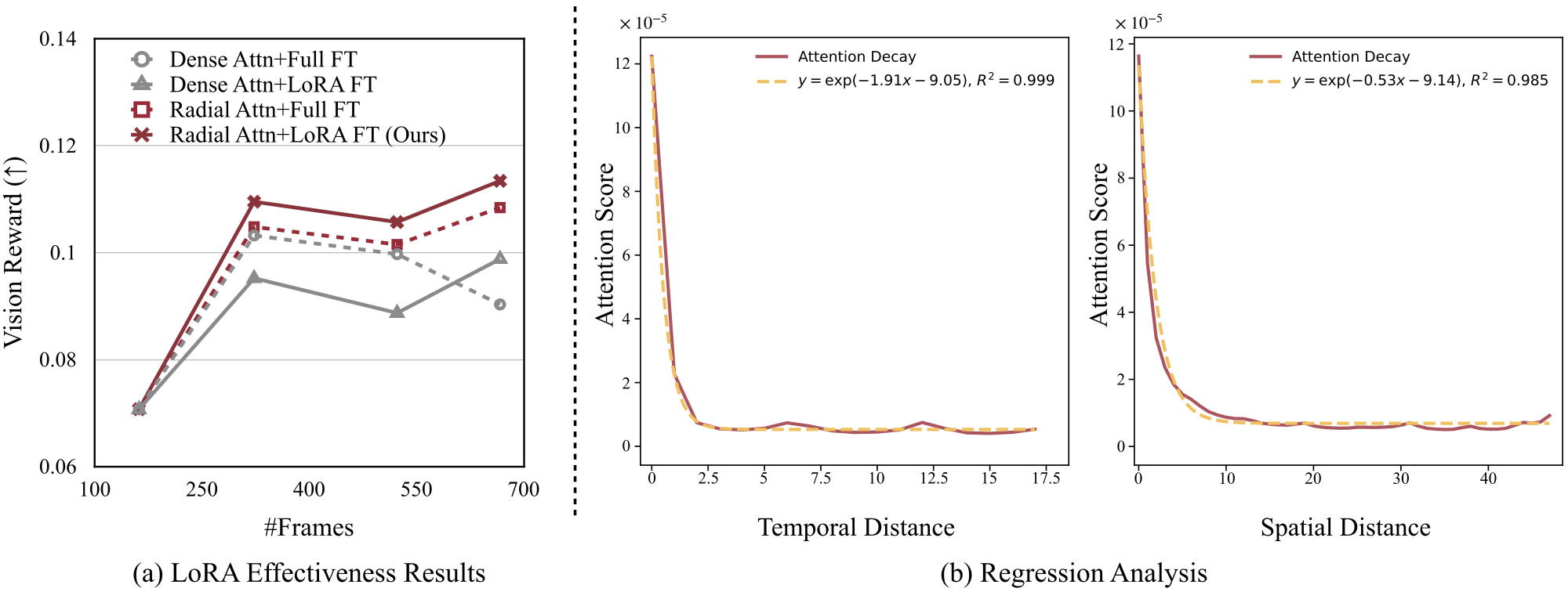
Figure 11 解读：(a) LoRA vs Full FT 的效果对比。Dense attention 下 LoRA 在 4x 长度时明显落后于 Full FT；但 Radial Attention 下 LoRA fine-tuning 反而匹配甚至超越 Full FT，说明 Radial Attention 使得模型更容易通过 LoRA 适配长视频。(b) Regression Analysis：用 y = exp(-ax + b) 拟合 attention score 的衰减曲线，temporal 和 spatial 两个方向的 R^2 均超过 0.985，验证了指数衰减假设。

Attention Error 对比

Method	Attention MSE
Radial Attention	3.9 x 10^-3
SVG	4.4 x 10^-3
STA	1.5 x 10^-2

与 Style LoRA 的兼容性

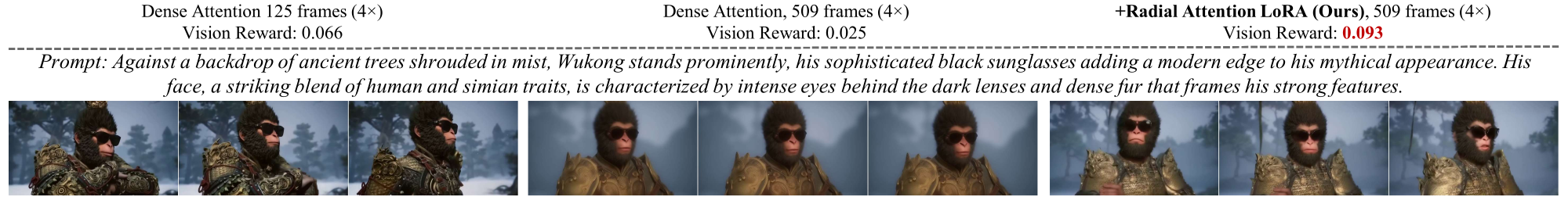
Figure 12 解读：Radial Attention 可以与现有的 style LoRA（如艺术风格迁移）无缝兼容。通过直接 merge Radial Attention 的 length-extension LoRA 和 style LoRA 的权重，可以同时实现长视频生成和风格化，无需额外训练。

其他模型上的结果

Mochi 1：

• 默认长度（163 帧）：加速推理至可用
• 2x 扩展（331 帧）：Sparsity 76.4%, 推理 1.63x, Vision Reward 0.110（最优）
• 4x 扩展（667 帧）：Sparsity 85.5%, 推理 2.57x, Vision Reward 0.113（最优）

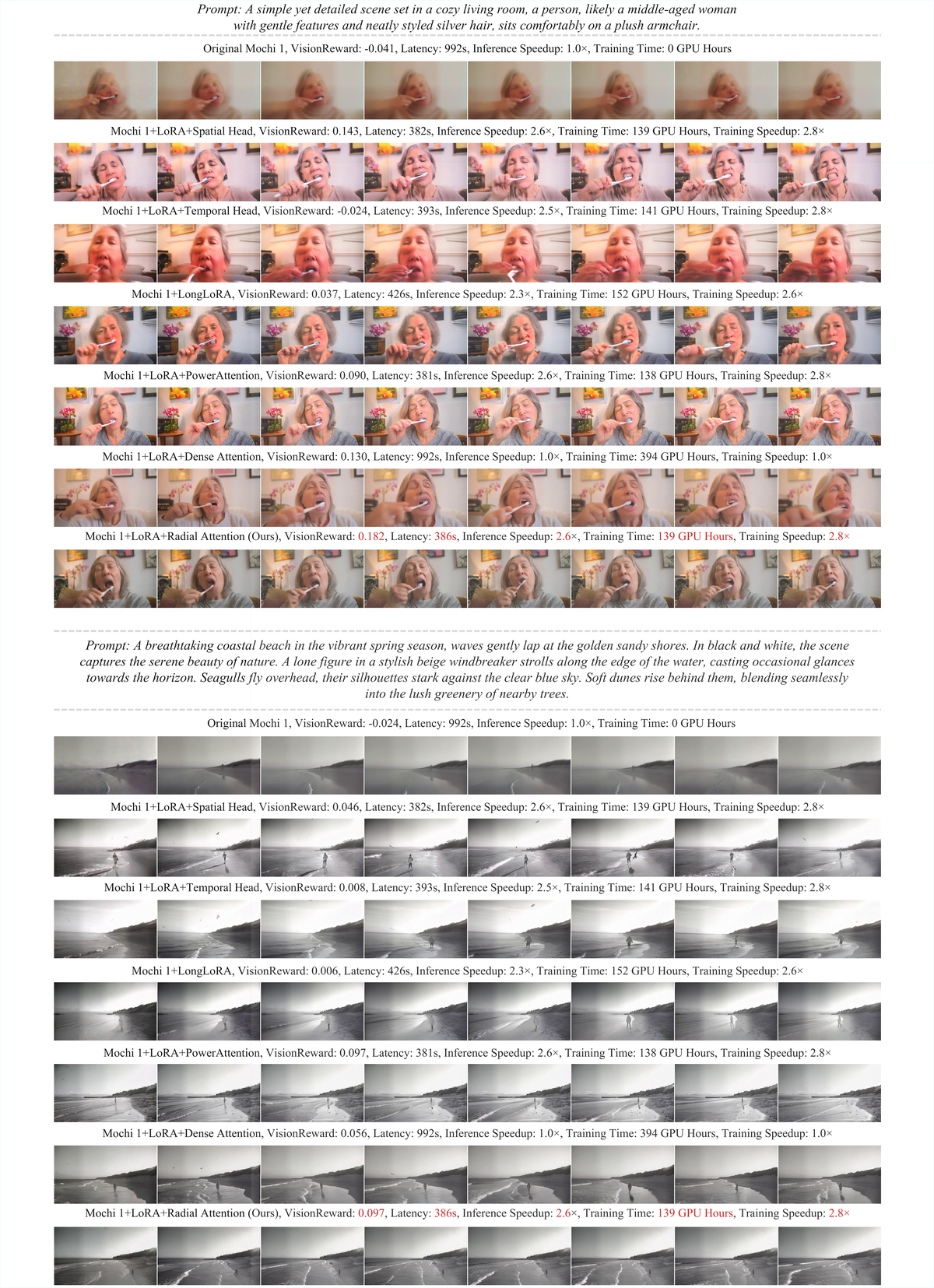
Figure 13 解读：Mochi 1 4x 扩展视觉对比。667 帧长视频生成。Radial Attention 在 Mochi 1 上同样实现了高质量的长视频生成，Vision Reward 达到所有方法中最优的 0.113，推理加速 2.57x。

Wan2.1-14B：

• 2x 扩展（161 帧）：Sparsity 73.6%, 推理 2.01x, Vision Reward 0.145（最优）

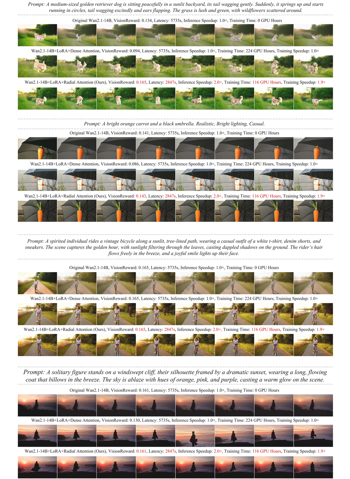
Figure 14 解读：Wan2.1-14B 2x 扩展视觉对比。161 帧长视频生成。Radial Attention + LoRA 以 73.6% sparsity 实现 2.01x 推理加速，Vision Reward 0.145 为所有方法最优。

Limitations

1. 假设 attention score 的指数衰减简化了自然视频数据中复杂的时空依赖关系
2. 方法对 spatial resolution 仍具有二次复杂度（O(n log n) 中 n = f*s，对 s 的复杂度为 O(s^2)）
3. 当前实现使用 FA2 backend，升级到 FA3 有望进一步加速