HiAR: Efficient Autoregressive Long Video Generation via Hierarchical Denoising

Authors: Kai Zou, Dian Zheng, Hongbo Liu, Tiankai Hang, Bin Liu, Nenghai Yu Affiliations: University of Science and Technology of China (USTC), The Chinese University of Hong Kong, Tongji University, Tencent Hunyuan, Anhui Province Key Laboratory of Digital Security (USTC) arXiv: 2603.08703 Project Page: jacky-hate.github.io/HiAR GitHub: Jacky-hate/HiAR Year: 2026

1. Motivation (研究动机)

自回归 (AR) 视频扩散模型能够生成理论上无限长的视频，但面临一个核心矛盾：

时序连续性 vs. 质量退化：现有 AR 方法（如 Self-Forcing）在生成下一个 block 时，将前一个 block 完全去噪至 $t_{c} = 0$ （即 clean context）作为条件。虽然 clean context 提供了最大的条件信号，但同时也以最大置信度传播了累积预测误差 $δ^{(n - 1)}$ ，导致逐 block 的分布漂移（color shift、over-saturation、motion repetition 等）。
核心洞察：作者指出 高度 clean 的 context 并非必要条件。双向扩散模型（如 Wan2.1）在相同噪声水平下对所有帧联合去噪，仍能保持时序连贯性。这说明 noisy context 已经提供了足够的条件信号，且能有效衰减误差传播。
最优噪声水平分析：context 噪声水平 $t_{c}$ 控制一个 bias-information trade-off。将 context 呈现为 $t_{c} = t_{j + 1}$ （当前去噪步的输出噪声水平）是满足时序因果性的最噪条件，在最大化误差衰减的同时保留所有必要的条件信息。

2. Idea (核心思想)

HiAR 提出 Hierarchical Denoising（分层去噪），将传统 AR 的 “block-first” 生成顺序翻转为 “step-first”：

去噪顺序翻转：不再逐 block 完成所有去噪步，而是在每个去噪步内对所有 block 执行因果生成。这样每个 block 的 context 自然处于与自身相同的噪声水平 $t_{j + 1}$ ，实现了误差衰减。
流水线并行：在 $N \times S$ 的 (block, step) 网格中，同一反对角线上的 $(n, j)$ 位置互相独立，可以分配到不同 GPU 实现 pipelined parallelism，获得 $\sim 1.8 \times$ wall-clock 加速。
Forward-KL 正则化：self-rollout distillation 在 hierarchical denoising 下会放大 reverse-KL 固有的 low-motion shortcut。作者引入 forward-KL regulariser，在 bidirectional-attention 模式下计算，保持运动多样性而不干扰 causal DMD 目标。

3. Method (方法)

3.1 整体框架

Figure 2 解读：左侧为现有 AR rollout（如 Self-Forcing），按 block-first 顺序逐 block 完成所有去噪步，每步条件化于 clean context（ $t_{c} = 0$ ），放大误差传播。右侧为 HiAR 的 hierarchical denoising，按 step-first 顺序在每个去噪步内对所有 block 因果生成，context 处于匹配的噪声水平 $t_{j + 1}$ 。下方为训练流程：causal rollout 结合 reverse-KL (DMD) loss，加上在 bidirectional-attention 模式下计算的 forward-KL regulariser 以保持运动多样性。

3.2 Context Noise Level 与误差传播分析

误差分解：考虑 block $B_{n}$ 在步骤 $j$ （从 $t_{j}$ 去噪到 $t_{j + 1}$ ）。设 $x_{0}^{(n - 1)}$ 为前一 block 的 ground-truth clean latent， $\overset{x}{^}_{0}^{(n - 1)} = x_{0}^{(n - 1)} + δ^{(n - 1)}$ 为模型预测。Context 在噪声水平 $t_{c} \in [0, 1]$ 下构造为：

c_{n - 1}^{(t_{c})} = (1 - σ_{t_{c}}) \overset{x}{^}_{0}^{(n - 1)} + σ_{t_{c}} η, η \sim N (0, I)

展开后分解为三项：

c_{n - 1}^{(t_{c})} = true signal (1 - σ_{t_{c}}) x_{0}^{(n - 1)} + propagated bias (1 - σ_{t_{c}}) δ^{(n - 1)} + stochastic perturbation σ_{t_{c}} η

真实信号和传播偏差共享系数 $(1 - σ_{t_{c}})$ ，随机扰动系数为 $σ_{t_{c}}$
$t_{c}$ 控制 bias-information trade-off：增大 $t_{c}$ 衰减偏差但同时减少有用条件信号
当 $t_{c} = 0$ （Self-Forcing 做法），误差无衰减直接传播

时序因果性约束：context 必须至少包含当前 block 在步骤 $j$ 后所拥有的信息量。SNR 单调递增要求：

SNR (t_{c}) \geq SNR (t_{j + 1}) ⟺ t_{c} \leq t_{j + 1}

最优选择：取约束边界即最噪条件：

t_{c}^{*} = t_{j + 1}

# Pseudocode: Context noise level selection
def get_context_noise_level(step_j, schedule):
    """Optimal context noise = output noise level of current step."""
    # schedule: [t_1=1, t_2, ..., t_S≈0]
    t_j = schedule[step_j]          # input noise level
    t_j1 = schedule[step_j + 1]    # output noise level
    # Optimal: use output level (noisiest that preserves causality)
    t_c = t_j1
    return t_c

3.3 Hierarchical Denoising 推理

核心改变：将去噪步 $j$ 放在外循环，block $n$ 放在内循环。每步中，block $B_{n}$ 以 $B_{< n}$ 在噪声水平 $t_{j + 1}$ 下的状态为 context。

Algorithm 1 — Hierarchical Denoising:

def hierarchical_denoising(model, schedule, initial_noise, N):
    """
    Args:
        model: denoiser v_theta
        schedule: [t_1=1, t_2, ..., t_S≈0], S denoising steps
        initial_noise: {x_t1^(n)} for n=1..N
        N: number of blocks
    Returns:
        generated blocks {x_hat_0^(n)} for n=1..N
    """
    S = len(schedule) - 1
    x = initial_noise  # x[n] = x_{t_1}^{(n)}
 
    for j in range(S):  # denoising steps (outer loop)
        t_j = schedule[j]
        t_j1 = schedule[j + 1]
        sigma_j = get_sigma(t_j)
        sigma_j1 = get_sigma(t_j1)
 
        for n in range(N):  # causal block sweep (inner loop)
            # Context: blocks B_{<n} at noise level t_{j+1}
            context = get_kv_cache(blocks[:n])
            # Euler step
            v_pred = model(x[n], t_j, context=context)
            x[n] = x[n] + v_pred * (sigma_j1 - sigma_j)
            # Update KV cache with x[n] at t_{j+1}
            update_kv_cache(n, x[n])
 
    return {n: x[n] for n in range(N)}

3.4 Pipelined Parallelism

Figure: Pipeline Parallelism 解读：在 $N \times S$ 网格中，block $B_{n}$ 在步骤 $j$ 仅依赖 $B_{< n}$ 在步骤 $j$ 以及 $B_{n}$ 在步骤 $j - 1$ 的结果。同一反对角线上的位置互相独立，可分配给不同 GPU。每个 stage 负责一个去噪步，stage 间通过异步点对点通信交换中间 latent。

KV cache 融合优化：在因果 attention 下，更新 $B_{n}$ 的 KV cache 和去噪 $B_{n + 1}$ 可融合为一次 forward call，将每 stage 的 forward pass 从 $2 N$ 减少到 $N + 2$ （第一个 block 单独去噪 + $N - 1$ 次融合 + 1 次尾部 cache 写入），在 4-step 设置下实现 $\sim 1.8 \times$ 加速。

# Pseudocode: DAC (Denoise-AddNoise-Cache) pipeline parallel
def pipeline_parallel_inference(model, schedule, noise, N, rank, world_size):
    """
    Each rank handles one denoising step (stage).
    Diagonal traversal of (block, step) grid.
    """
    S = len(schedule) - 1
    assert world_size == S  # one GPU per denoising step
 
    for diag in range(N + S - 1):
        n = diag - rank  # block index for this rank
        if 0 <= n < N:
            j = rank  # this rank's denoising step
            t_j, t_j1 = schedule[j], schedule[j + 1]
 
            # Receive x[n] at t_j from previous stage
            if rank > 0:
                x_n = recv(src=rank - 1)
            else:
                x_n = noise[n]
 
            # Phase D: Denoise
            v_pred = model(x_n, t_j, context=kv_cache[:n])
            x_denoised = x_n + v_pred * (sigma(t_j1) - sigma(t_j))
 
            # Phase A: Send to next stage (overlapped)
            if rank < world_size - 1:
                send(x_denoised, dst=rank + 1)
 
            # Phase C: Update KV cache (overlapped with next stage's D)
            update_kv_cache(n, x_denoised)

3.5 Training with Forward-KL Regulation

训练采用 self-rollout distillation，在 hierarchical denoising pipeline 下进行。

DMD Loss (Reverse-KL)：student model $v_{θ}$ 先 rollout 生成 $\overset{x}{^}_{0}^{(n - 1)}$ ，再用作下一 block 的 context。训练目标为 reverse-KL (DMD)：

L_{DMD} = E_{t, x_{t}} [D_{KL} (p_{θ} (x_{0} ∣ x_{t}) ∥ p_{teacher} (x_{0} ∣ x_{t}))]

Low-motion shortcut 问题：reverse-KL 的 mode-seeking 性质使 student 倾向于生成低运动输出以最小化 loss。Hierarchical denoising 放大了此效应，因为条件化于多水平 noisy context 增加了学习难度，给 mode-seeking 目标更多迭代以收敛到低运动模式。

Forward-KL Regulariser：从 teacher 采样 dense denoising trajectory ${x_{t_{1}}^{ref}, \dots, x_{t_{S}}^{ref}}$ ，监督 student 匹配相邻步之间的 velocity：

L_{FKL} = E_{t} v_{θ} (x_{t_{i}}^{ref}, t_{i}) - \frac{x _{t_{i + 1}}^{ref} - x _{t_{i}}^{ref}}{σ _{t_{i + 1}} - σ _{t_{i}}}^{2}

因为 target $x_{t}^{ref}$ 来自 teacher 分布，优化此目标等价于最小化 forward-KL，鼓励 student 覆盖 teacher 的输出模式，保持运动多样性。

解耦设计：

仅 bidirectional-attention 模式： $L_{FKL}$ 仅在 bidirectional-attention 下计算，不修改 causal self-rollout DMD loss。因为 bidirectional 和 causal 模式下的 motion dynamics 强正相关（Pearson $r = 0.968$ ），正则化前者等效约束后者。
仅前 $K$ 步：motion dynamics 主要由低频结构决定（earliest denoising steps），因此 $L_{FKL}$ 仅应用于前 $K = 1$ 步。

总训练目标：

L = L_{DMD} + λ L_{FKL}

其中 $λ = 0.1$ ，critic 和 generator 以 5:1 比例交替更新。

# Pseudocode: HiAR training step
def train_step(student, teacher, critic, batch, ode_pairs):
    """
    Combined DMD + Forward-KL training.
    Args:
        student: student generator v_theta
        teacher: frozen teacher (Wan2.1-1.3B)
        critic: fake score network (Wan2.1-14B)
        batch: training data with text prompts
        ode_pairs: pre-sampled teacher ODE trajectories
    """
    # === Phase 1: DMD Loss (causal rollout) ===
    # Self-rollout under hierarchical denoising
    x_gen = hierarchical_rollout(student, batch, causal_attention=True)
    # Compute reverse-KL gradient via critic
    dmd_loss = compute_dmd_loss(student, critic, x_gen, batch)
 
    # === Phase 2: Forward-KL Loss (bi-attn mode) ===
    # Sample teacher trajectory pair (x_ti, x_ti+1)
    x_ref_t, x_ref_t1, t_i, t_i1 = sample_ode_pair(ode_pairs)
    # Student prediction in bidirectional-attention mode
    v_pred = student(x_ref_t, t_i, bidirectional_attention=True)
    # Target velocity from teacher trajectory
    v_target = (x_ref_t1 - x_ref_t) / (sigma(t_i1) - sigma(t_i))
    fkl_loss = mse_loss(v_pred, v_target)
 
    # === Combined objective ===
    lambda_fkl = 0.1
    total_loss = dmd_loss + lambda_fkl * fkl_loss
    total_loss.backward()

Figure 4 解读：训练过程中 bidirectional dynamic score 与 causal dynamic score 的相关性散点图。每个点代表一个 training checkpoint，颜色编码训练步数。Pearson $r = 0.968$ 的强正相关证实 low-motion shortcut 同时影响两种 attention 模式，正则化 bidirectional 模式能有效约束 causal 模式的运动多样性。

3.6 Code-to-Paper 映射表

Paper Concept	Source File	Key Class/Function
Hierarchical Denoising 推理	`pipeline/causal_inference.py`	`CausalInferencePipeline.inference()`
Timestep-first training loop	`pipeline/timestep_forcing_training.py`	`TimestepForcingTrainingPipeline._timestep_first_loop()`
Frame-first training loop	`pipeline/timestep_forcing_training.py`	`TimestepForcingTrainingPipeline._frame_first_loop()`
DMD loss (Reverse-KL)	`model/dmd.py`	`DMD.compute_distribution_matching_loss()`
Forward-KL regulariser ( $L_{FKL}$ )	`model/timestep_forcing_dmd.py`	`TimestepForcingDMD.progressive_distillation_loss()`
KV cache 融合 forward	`model/timestep_forcing_dmd.py`	`TimestepForcingDMD._pd_single_forward()`
Pipeline parallel inference (DAC)	`scripts/pipeline_parallel_inference.py`	`_run_dac()`
Pipeline parallel inference (baseline)	`scripts/pipeline_parallel_inference.py`	`_run_baseline()`
Critic loss	`model/dmd.py`	`DMD.critic_loss()`
Generator loss	`model/dmd.py`	`DMD.generator_loss()`
训练主循环	`trainer/distillation.py`	`DistillationTrainer.train()`, `fwdbwd_one_step()`
Teacher ODE trajectory 生成	`scripts/generate_ode_pairs.py`	—
Noise schedule ( $σ_{t}$ )	`wan/utils/fm_solvers.py`	—

4. Experimental Setup (实验设置)

Base model: Wan2.1-1.3B，teacher 为 Wan2.1-14B

训练配置：

4-step denoising schedule ( $S = 4$ )
Chunk-wise 实现，每 chunk 3 个 latent frames
16k ODE solution pairs，causal attention masking fine-tune
Forward-KL：从 Wan2.1-1.3B base model 采样 20k denoising trajectories（50 ODE steps each），仅约束第 1 个去噪步 ( $K = 1$ )， $λ = 0.1$
Learning rate: $2 \times 1 0^{- 6}$ ，batch size 64，训练 20k steps on 5-second clips
推理时使用 sliding-window KV cache（5s window）

评测指标：

VBench：16 维度，分为 Quality score 和 Semantic score，所有模型采样 20s
Drift Score（本文提出）：将 20s 视频均分为 5 段，计算每段的感知质量（MUSIQ、CLIP-IQA）、时序连贯性（DINOv2 cosine similarity、LPIPS）、低级统计量（HSV saturation mean、Laplacian variance），对每个指标做线性回归取斜率，归一化加权求和

Baselines：

双向扩散：LTX-Video、Wan2.1-1.3B
AR 扩散：NOVA、Pyramid Flow、SkyReels-V2 (1.3B)、MAGI-1 (4.5B)
Distilled AR：CausVid、Self-Forcing、Causal Forcing

5. Experimental Results (实验结果)

5.1 主实验 (Table 1: 20s generation)

Model	Thru. (fps)	Lat. (s)	Total↑	Quality↑	Semantic↑	Dynamic↑	Drift↓
LTX-Video	8.98	13.5	0.766	0.789	0.685	0.458	–
Wan2.1-1.3B	0.78	103	0.802	0.813	0.766	0.690	–
NOVA	0.88	4.1	0.773	0.777	0.757	0.444	–
Pyramid Flow	6.70	2.5	0.775	0.804	0.670	0.161	–
SkyReels-V2 (1.3B)	0.49	112	0.788	0.808	0.707	0.333	–
MAGI-1 (4.5B)	0.19	282	0.757	0.785	0.647	0.486	–
CausVid	17	0.69	0.764	0.771	0.740	0.621	0.842
Self-Forcing	17	0.69	0.805	0.829	0.708	0.542	0.355
Causal Forcing	17	0.69	0.810	0.837	0.701	0.672	0.615
HiAR (Ours)	30	0.30	0.821	0.846	0.723	0.686	0.257

关键发现：

HiAR 在所有方法中取得最高 Total score (0.821)，最高 Quality score (0.846)，最低 Drift (0.257)
相比 Self-Forcing，Drift 降低 27.6%（0.257 vs. 0.355）
吞吐量 30 fps，per-chunk latency 0.30s，相比同 backbone 的 distilled AR 模型实现 $\sim 1.8 \times$ 加速
Dynamic score 0.686，接近 Wan2.1-1.3B teacher (0.690)，远超 Self-Forcing (0.542)

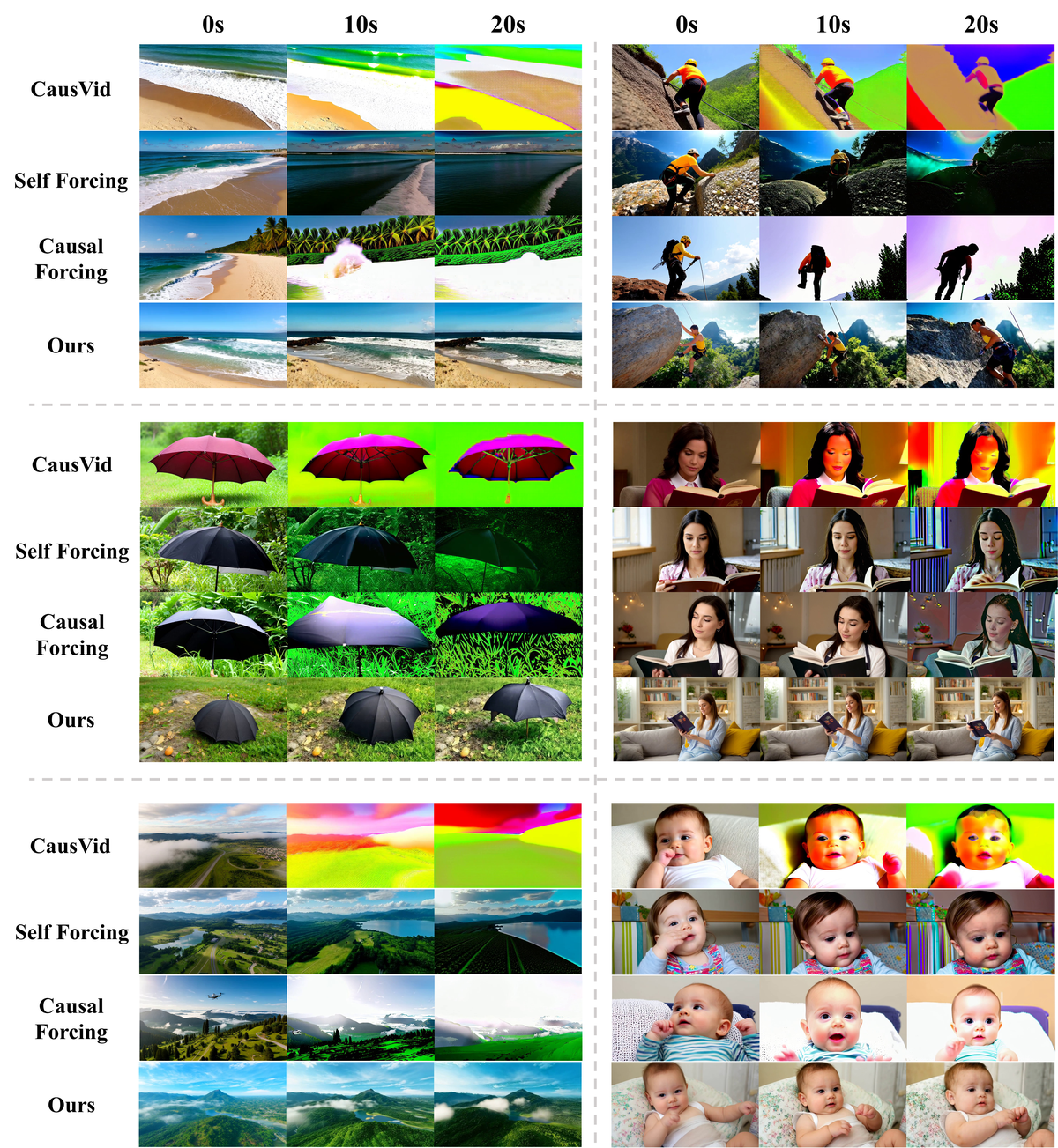
Figure 3 解读：distilled AR 模型在 20s 生成上的定性对比。CausVid 退化最严重（色调偏移至 neon green/yellow），Self-Forcing 和 Causal Forcing 存在明显的色彩过饱和。HiAR 在所有 prompt 类型上保持稳定的色彩保真度和结构连贯性，无可感知的 drift。

5.2 Ablation: Context Noise Level (Table 2)

Context noise $t_{c}$	Quality↑	Semantic↑	Smooth.↑	Drift↓
$t_{c} = t_{j}$ (input level)	0.799	0.692	0.978	0.184
$t_{c} = t_{j + 1}$ (output level; default)	0.846	0.723	0.988	0.257
$t_{c} = 0$ (Self-Forcing)	0.829	0.708	0.991	0.355

$t_{c} = t_{j}$ ：最低 drift (0.184) 但质量显著下降 (0.799)，运动不流畅 (Smooth 0.978)
$t_{c} = t_{j + 1}$ （HiAR default）：最佳质量-稳定性平衡
$t_{c} = 0$ （Self-Forcing）：最高 drift (0.355)

5.3 Ablation: Forward-KL Regulariser Design (Table 3)

Configuration	Quality↑	Semantic↑	Dynamic↑	Drift↓
bi-attn + 1 step (default)	0.846	0.723	0.686	0.257
causal + 1 step	0.828	0.701	0.625	0.271
bi-attn + 2 steps	0.835	0.708	0.693	0.296
bi-attn + 4 steps	0.813	0.684	0.691	0.306
w/o $L_{FKL}$	0.839	0.732	0.445	0.218
w/o re-training	0.767	0.559	0.512	0.309
w/o hier. denoising (Self-Forcing)	0.829	0.708	0.542	0.355

去除 $L_{FKL}$ ：Dynamic 暴跌至 0.445，确认 low-motion shortcut 的存在
仅推理时使用 hierarchical denoising (w/o re-training)：Drift 改善 (0.309 vs. 0.355) 但质量损失大 (0.767)
Causal 模式下的 $L_{FKL}$ 效果弱于 bidirectional 模式 (Dynamic 0.625 vs. 0.686)
增加约束步数 $K$ 带来的 Dynamic 边际收益递减但质量和 drift 恶化

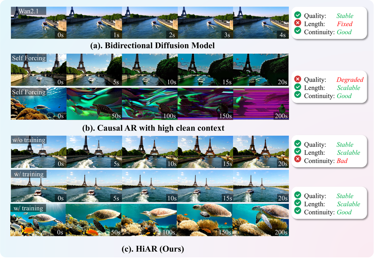
Figure 1 解读：Motivation 总览。(a) Bidirectional diffusion（Wan2.1）证明 shared noise level 下即可保持时序连贯，但长度固定。(b) 标准 AR（Self-Forcing）可扩展长度但 clean context 导致质量退化。(c) HiAR 的 hierarchical denoising 在推理时（w/o training）即可缓解 drift，经过重训练（w/ training）后实现稳定质量、可扩展长度和无缝连续性。

Paper Notes

探索

HiAR: Efficient Autoregressive Long Video Generation via Hierarchical Denoising

HiAR: Efficient Autoregressive Long Video Generation via Hierarchical Denoising

1. Motivation (研究动机)

2. Idea (核心思想)

3. Method (方法)

3.1 整体框架

3.2 Context Noise Level 与误差传播分析

3.3 Hierarchical Denoising 推理

3.4 Pipelined Parallelism

3.5 Training with Forward-KL Regulation

3.6 Code-to-Paper 映射表

4. Experimental Setup (实验设置)

5. Experimental Results (实验结果)

5.1 主实验 (Table 1: 20s generation)

5.2 Ablation: Context Noise Level (Table 2)

5.3 Ablation: Forward-KL Regulariser Design (Table 3)

目录