Diffusion Adversarial Post-Training for One-Step Video Generation

Authors: Shanchuan Lin, Xin Xia, Yuxi Ren, Ceyuan Yang, Xuefeng Xiao, Lu Jiang Affiliations: ByteDance Seed arXiv: 2501.08316 Project Page: seaweed-apt.com Venue: ICML 2025 Code: 未开源 (相关后续工作 SeedVR2 已开源)

1. Motivation (研究动机)

1.1 核心问题

Diffusion model 的迭代采样过程非常缓慢, 生成高分辨率视频 (如 1280x720, 24fps, 2秒) 在 H100 上需要数分钟。现有的 diffusion step distillation 方法存在以下问题:

质量显著下降: 现有 distillation 方法在 one-step 生成时质量严重退化, 特别是在细节、结构完整性和文本对齐方面
视频生成受限: 已有工作仅在小规模低分辨率视频 (512x512, 16帧) 上进行蒸馏, 高分辨率视频的 one-step 生成此前尚未实现
蒸馏范式的局限: 传统 distillation 方法以预训练 diffusion model 为 teacher, 生成的质量天然受限于 teacher 的上限

1.2 关键洞察

作者提出了一个不同于 distillation 的范式: Adversarial Post-Training (APT) — 不再将预训练的 diffusion model 作为 teacher 来蒸馏, 而是仅将其作为初始化, 然后直接对 real data 进行 adversarial training。这类似于 supervised fine-tuning (SFT) 在 post-training 阶段的角色。

这带来两个关键优势:

省去了预计算大量 teacher 样本的成本
生成质量不再受限于 teacher, 在 visual fidelity 上甚至可以超越 25-step diffusion model

2. Idea (核心思想)

核心思路: 将 text-to-video diffusion model 转化为 one-step generator, 通过在 diffusion pre-training 之后追加 adversarial post-training 阶段, 直接对 real data 进行 GAN-style 训练。

具体来说:

先用 consistency distillation 初始化 generator (提供粗略的 one-step 能力)
用预训练 diffusion model 权重初始化 discriminator (共享相同的 DiT 架构)
在 real data 上进行标准 adversarial training, 配合近似 R1 regularization 保证训练稳定性

这是目前报道的最大规模 GAN (~16B 参数), 同时支持 image 和 video 生成。

3. Method (方法)

3.1 总体架构

Figure 1 解读: 左侧是 Generator Transformer (36层), 从 consistency model 初始化; 中间是 Discriminator Transformer (36层), 从原始 diffusion model 初始化。两者共享相同的 MMDiT 架构。右侧展示了 discriminator 的额外 output head: 在第16、26、36层添加 cross-attention-only transformer block, 用单个 learnable token 作为 query, 对所有 visual token 做 cross-attend, 产生 scalar logit。多层 feature 的 channel-concatenation 最终产生标量输出。

3.2 Generator

Generator 的初始化分两步:

Step 1: Consistency Distillation 初始化

首先用 consistency distillation (Song et al., 2023; Song & Dhariwal, 2024) 配合 MSE loss 预训练一个基础的 one-step 模型 $\hat{G}$ :

\overset{v}{^} = \hat{G} (z, c, T)

\overset{x}{^} = z - \overset{v}{^}

其中 $z$ 是噪声, $c$ 是文本条件, $T$ 是最终 timestep, CFG scale 固定为 7.5。

Step 2: 定义 Generator

以 consistency model 为初始化, 定义 generator:

G (z, c) := z - \hat{G} (z, c, T)

即 generator 输出的是去噪后的 clean sample prediction。

# Pseudocode: Generator 初始化与前向
class Generator(nn.Module):
    def __init__(self, pretrained_consistency_model):
        self.dit = copy.deepcopy(pretrained_consistency_model)
 
    def forward(self, z, c):
        # z: noise sample, c: text condition
        # 固定 timestep 为 T (最终时刻)
        v_pred = self.dit(z, c, t=T)  # velocity prediction
        x_pred = z - v_pred           # clean sample prediction
        return x_pred

3.3 Discriminator

Discriminator 的设计包含三个关键决策:

1) 从 diffusion model 初始化 (非 consistency model)

实验发现用原始 diffusion 权重初始化效果更好。

2) Multi-layer feature aggregation

在第 16、26、36 层添加 cross-attention output head:

# Pseudocode: Discriminator multi-layer logit head
class DiscriminatorHead(nn.Module):
    def __init__(self, hidden_dim, num_layers=3):
        # 在 layer 16, 26, 36 各添加一个 cross-attention block
        self.cross_attn_blocks = nn.ModuleList([
            CrossAttentionBlock(hidden_dim) for _ in range(num_layers)
        ])
        self.learnable_query = nn.Parameter(torch.randn(1, 1, hidden_dim))
        self.proj = nn.Linear(hidden_dim * num_layers, 1)
 
    def forward(self, features_list):
        # features_list: [feat_16, feat_26, feat_36], 每个是 visual tokens
        tokens = []
        for feat, block in zip(features_list, self.cross_attn_blocks):
            # 单个 learnable token 做 query, visual tokens 做 key/value
            token = block(query=self.learnable_query, kv=feat)  # [B, 1, D]
            tokens.append(token)
        # Channel concatenation + projection
        concat = torch.cat(tokens, dim=-1)  # [B, 1, 3D]
        logit = self.proj(concat).squeeze()  # [B]
        return logit

3) Timestep ensemble (用不同 timestep 输入)

由于 discriminator 从 diffusion model 初始化, 而 diffusion model 在 $t = 0$ 时无意义, 所以对输入 timestep 做 ensemble:

D (x, c) := E_{t \sim shift (U (0, T), s)} [\hat{D} (x, t, c)]

其中 shift 函数为:

shift (t, s) := \frac{s \times t}{1 + ( s - 1 ) \times t}

$s$ 是由 latent 维度决定的超参数, image 用 $s = 1$ , video 用 $s = 12$ 。

# Pseudocode: Discriminator timestep ensemble
class Discriminator(nn.Module):
    def __init__(self, pretrained_diffusion_model):
        self.dit = copy.deepcopy(pretrained_diffusion_model)
        self.head = DiscriminatorHead(hidden_dim=dit.hidden_dim)
 
    def forward(self, x, c):
        # 采样随机 timestep 并做 shift
        t = torch.rand(1) * T  # uniform from [0, T]
        t_shifted = (s * t) / (1 + (s - 1) * t)
 
        # 前向 DiT, 收集多层 feature
        features = self.dit.forward_with_features(x, t_shifted, c,
                                                   extract_layers=[16, 26, 36])
        logit = self.head(features)
        return logit

直接输入 clean data: Discriminator 直接接收 clean sample $x$ 或 $\overset{x}{^}$ (不加噪), 而 timestep ensemble 是对 discriminator 内部的条件化。

3.4 Approximated R1 Regularization

标准 R1 regularization 需要二阶梯度:

L_{R 1} = ∥ \nabla_{x} D (x, c) ∥_{2}^{2}

但 PyTorch FSDP、gradient checkpointing、FlashAttention 等均不支持 double backward。作者提出近似 R1:

L_{a R 1} = ∥ D (x, c) - D (N (x, σ I), c) ∥_{2}^{2}

即用有限差分近似梯度: 对 real data 加小方差 ( $σ = 0.01$ for images, $σ = 0.1$ for videos) 高斯噪声, 鼓励 discriminator 在 real data 附近的预测平滑。

# Pseudocode: Approximated R1 Regularization
def approx_r1_loss(discriminator, x_real, c, sigma=0.01):
    """
    近似 R1: 不需要二阶梯度, 兼容 FSDP / FlashAttention
    核心思想: D(x) 应约等于 D(x + noise), 即 D 在 real data 附近平滑
    """
    # 对 real data 加小扰动
    x_perturbed = x_real + sigma * torch.randn_like(x_real)
 
    # 计算两者的 discriminator output 差异
    d_real = discriminator(x_real, c)
    d_perturbed = discriminator(x_perturbed, c)
 
    loss_ar1 = (d_real - d_perturbed).pow(2).mean()
    return loss_ar1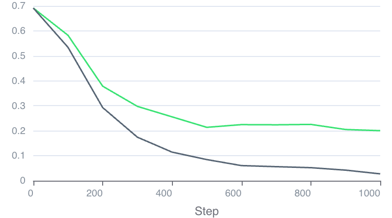

Figure 5 解读: 上图展示了有/无 approximated R1 regularization 的训练曲线对比。黑色曲线 (无正则化) 的 discriminator loss 快速降到零, 训练崩溃, generator 产出 mode collapse 的彩色色块。绿色曲线 (有正则化) 的 discriminator loss 保持健康水平, 不会降到零, 训练稳定。这证明 approximated R1 对于防止训练崩溃至关重要。

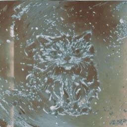
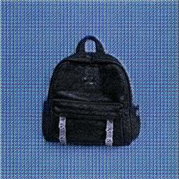
Figure 3 解读: 这组四张图展示了训练崩溃时生成器输出的彩色块状结果，对应无正则化情况下的 mode collapse 现象。

3.5 训练目标

Discriminator loss (使用 non-saturating GAN loss + approximated R1):

L_{D} = E_{x, c \sim T} [f_{D} (D (x, c))] + E_{z \sim N, c \sim T} [f_{G} (D (G (z, c), c))] + λ E_{x, c \sim T} [∥ D (x, c) - D (N (x, σ I), c) ∥_{2}^{2}]

其中 $f_{D} (x) = lo g σ (x)$ , $f_{G} (x) = lo g (1 - σ (x))$ , $λ = 100$ 。

Generator loss:

L_{G} = E_{z \sim N, c \sim T} [g_{G} (D (G (z, c), c))]

其中 $g_{G} (x) = lo g σ (x)$ 。

# Pseudocode: 完整训练循环
def train_step(generator, discriminator, real_batch, lambda_r1=100, sigma=0.01):
    x_real, c = real_batch  # real latent, text condition
 
    # === Discriminator step ===
    z = torch.randn_like(x_real)
    x_fake = generator(z, c).detach()
 
    d_real = discriminator(x_real, c)
    d_fake = discriminator(x_fake, c)
 
    # Non-saturating GAN loss
    loss_d = -F.logsigmoid(d_real).mean() - F.logsigmoid(-d_fake).mean()
 
    # Approximated R1
    x_perturbed = x_real + sigma * torch.randn_like(x_real)
    d_perturbed = discriminator(x_perturbed, c)
    loss_ar1 = (d_real - d_perturbed).pow(2).mean()
 
    loss_d_total = loss_d + lambda_r1 * loss_ar1
    loss_d_total.backward()
    optimizer_d.step()
 
    # === Generator step ===
    z = torch.randn_like(x_real)
    x_fake = generator(z, c)
    d_fake = discriminator(x_fake, c)
 
    loss_g = -F.logsigmoid(d_fake).mean()
    loss_g.backward()
    optimizer_g.step()
 
    # EMA update
    ema_update(generator_ema, generator, decay=0.995)

3.6 训练细节

阶段	数据	GPU	Batch Size	LR	训练步数	EMA
Image APT	1024px images	128~256 H100	9062	5e-6	350 (EMA)	decay=0.995
Video APT	1280x720, 24fps, 2s	1024 H100	2048	3e-6	300	decay=0.995

Optimizer: RMSProp ( $α = 0.9$ ), 等价于 Adam ( $β_{1} = 0, β_{2} = 0.9$ ), 比标准 Adam 节省显存
训练精度: BF16 mixed precision
Video 阶段的 generator 从 image EMA checkpoint 初始化, discriminator 重新从 diffusion weights 初始化
无 weight decay, 无 gradient clipping

4. Experimental Setup (实验设置)

4.1 Base Model

基于 Seaweed-7B (Seawead et al., 2025) — 一个基于 MMDiT 架构的 text-to-video diffusion model:

36 层 transformer blocks, 共 8B 参数
Flow matching objective (Lipman et al., 2023)
在 latent space 中操作 (Rombach et al., 2021)
支持任意分辨率的图片和视频生成

4.2 评估

Image 评估:

300 randomly selected prompts from PartiPrompt + DrawBench
3 images per prompt
Baseline: FLUX-Schnell, SD3.5-Turbo, SDXL-DMD2, SDXL-Hyper, SDXL-Lightning, SDXL-Nitro-Realism, SDXL-Turbo

Video 评估:

96 custom prompts, 1 video per prompt
VBench metrics
与 25-step diffusion baseline 对比

User Study: 3 个评价维度 — visual fidelity, structural integrity, text alignment, 共 50,328 sample comparisons。

5. Experimental Results (实验结果)

5.1 Image 定性结果

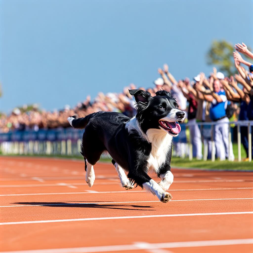
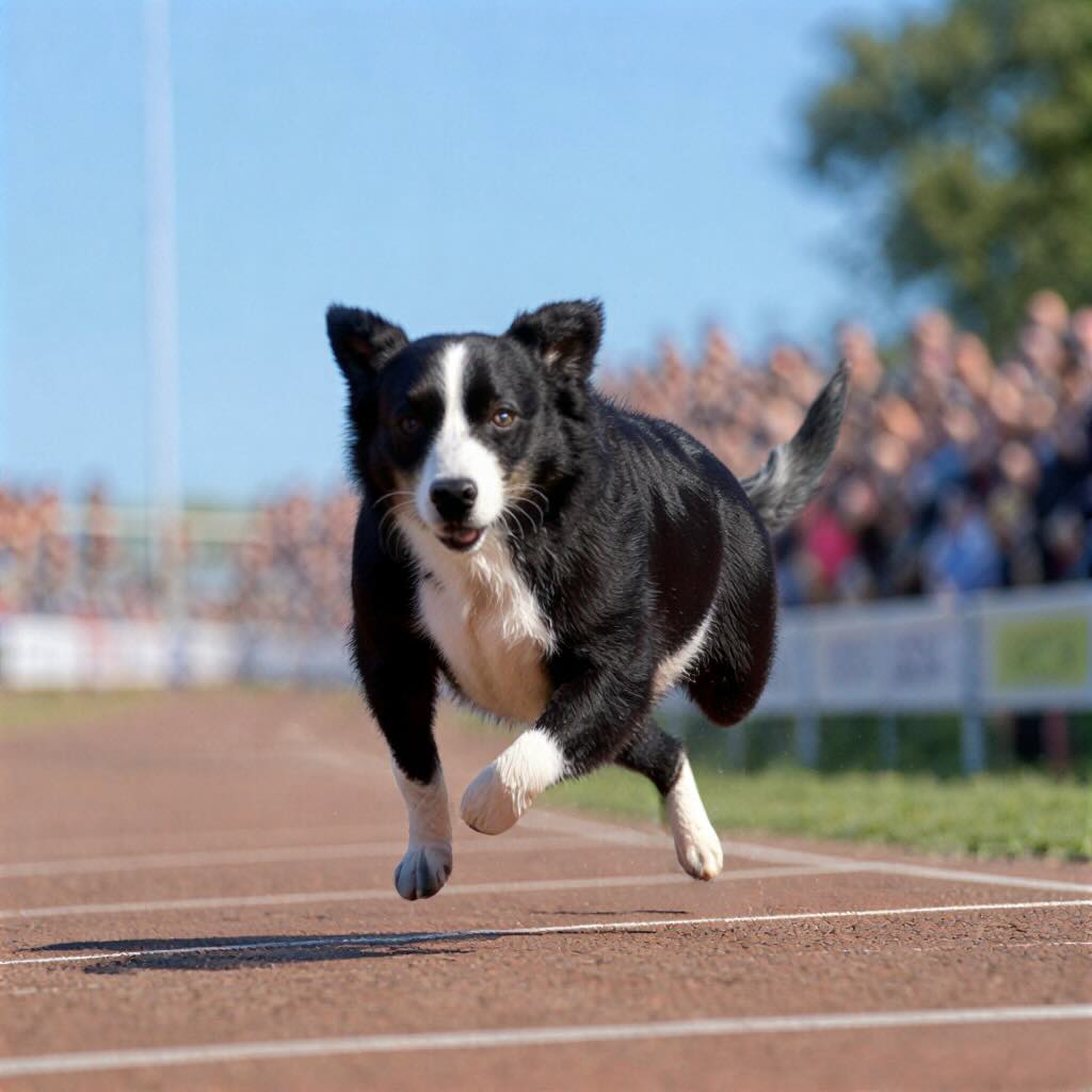
Figure 2 解读: 左侧是 25-step diffusion + CFG 的结果, 右侧是 1-step APT 的结果。APT 生成的图像色调更真实自然 (diffusion + CFG 容易过曝和过饱和), 细节更丰富。这是 APT 超越 teacher 的直观证据 — 因为它直接从 real data 学习, 而非受限于 CFG 产生的 synthetic 分布。

5.2 Image 定量结果 (User Study)

Table 1: One-Step vs. 25-Step Diffusion

Method	Visual Fidelity	Structural Integrity	Text Align
FLUX-Schnell	-36.6%	-24.4%	-2.8%
SD3.5-Large-Turbo	-94.4%	-30.1%	-20.4%
SDXL-DMD2	-9.3%	-16.8%	-4.6%
APT (Ours)	+37.2%	-13.1%	-8.1%

APT 是唯一在 visual fidelity 上超越 25-step diffusion 的 one-step 方法 (+37.2%), 但在 structural integrity 和 text alignment 上仍有退化。

Table 2: vs. SOTA One-Step Methods (Absolute Preference)

Method	Visual Fidelity	Structural Integrity	Text Align	Average
FLUX-Schnell	+35.7%	-21.5%	-28.1%	-4.6%
SDXL-DMD2	+34.7%	+10.3%	-11.8%	+11.1%
SDXL-Lightning	+34.1%	+14.1%	+11.4%	+19.9%
SDXL-Turbo	+68.9%	+14.9%	-7.9%	+25.3%

APT 在 absolute preference 上排名第二 (仅次于 FLUX-Schnell), relative preference 排名第一。Visual fidelity 全面领先所有方法。

5.3 Video 结果

Figure 4 解读: 上排为 25-step diffusion (50 NFE), 中排为 2-step APT (2 NFE), 下排为 1-step APT (1 NFE)。APT 在好的 case 中增强了细节和真实感。但 one/two-step 模型在 structural integrity 和 text alignment 上仍不如 25-step。

Table 4: Video User Study

Method	Steps	Visual Fidelity	Structural Integrity	Text Align
APT	2	+32.3%	-31.3%	-9.4%
APT	1	+10.4%	-38.5%	-8.3%

Table 7: VBench Metrics

Method	Steps	Total Score	Quality Score	Semantic Score
Diffusion	25	82.15	84.36	73.31
Consistency	1	67.05	73.78	40.15
APT	1	82.00	84.21	73.15

APT 1-step 的 VBench total score (82.00) 接近 25-step diffusion (82.15), 远超 consistency baseline 1-step (67.05)。

5.4 推理速度

Table 8: Inference Speed (1280x720, 24fps, 2s video)

H100 数量	Text Encoder	DiT	VAE	Total
1	0.28s	2.65s	3.10s	6.03s
4	0.28s	0.73s	1.19s	2.20s
8	0.28s	0.50s	1.19s	1.97s

8 张 H100 可实现实时 one-step 视频生成 (<2s 生成 2s 视频)。

5.5 Ablation Studies

Discriminator 深度: Full-depth (36层) > Two-thirds > Half-depth

Figure 6 解读: 从左到右分别是 half-depth (layer 14,16,18), two-thirds-depth (layer 18,22,26), full-depth (layer 16,26,36) discriminator 的生成结果。更深的 discriminator 利用了预训练网络的完整表征能力, 生成质量更高。

Multi-layer vs. Single-layer features:

Figure 7 解读: 左图仅使用最后一层 (layer 36) 的 discriminator, 右图使用多层 (layer 16,26,36) discriminator。多层 feature 显著提升了 structural correctness — 因为不同层捕获不同粒度的结构信息。

Training progression:

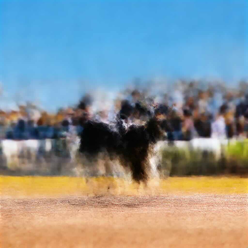
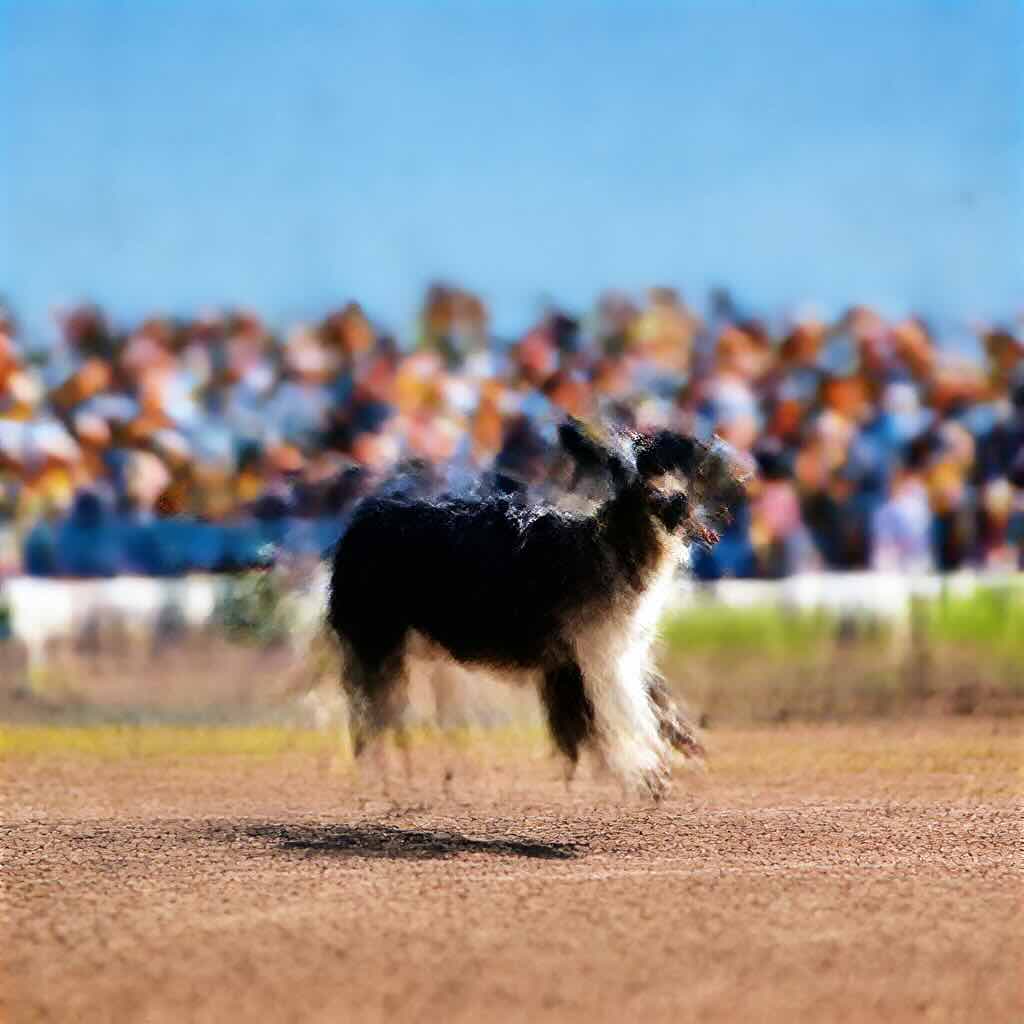
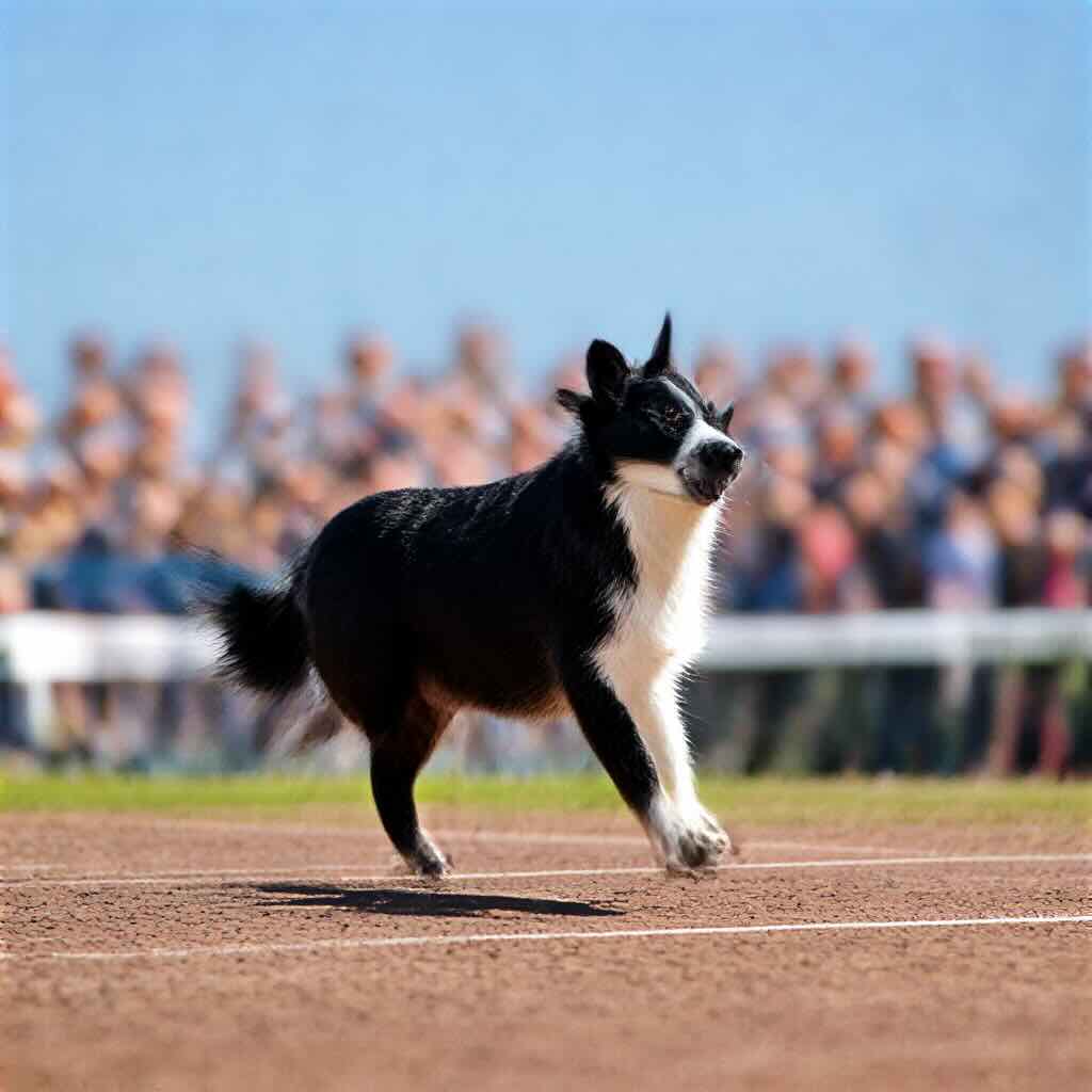
Figure 9 解读: 训练进度 (EMA model, 从左到右: 0, 1000, 2000, 3000, 5000, 7000, 8000, 10000 steps)。模型在约 50 步后就能生成清晰图像, EMA 模型在 350 步时质量达到峰值, 之后开始退化 (structural degradation 加剧)。

Batch size 对 video 的影响:

Figure 10 解读: 左图 batch size 256, 右图 batch size 1024。小 batch size 导致 mode collapse (不同 prompt 和 seed 产生相似结果), 大 batch size 避免了此问题。这与先前 GAN 研究中大 batch 有助于稳定性的结论一致。

Learning rate 策略:

Figure 11 解读: 从左到右: freeze backbone (只训新参数), 降低 backbone LR, 全参数相同 LR。Freeze backbone 产生不自然 artifacts, 低 LR 收敛太慢, 全参数相同 LR 效果最好。

5.6 Structural Degradation 分析

Figure 8 解读: Latent interpolation 实验显示, one-step generator 在 mode 之间的过渡区域容易出现 structural incorrectness。作者假设这是因为 generator 容量不足 (under-capacitated) — 36 层 transformer 要在单次前向中完成原本需要迭代 25 步的生成过程。这也是 text alignment 退化的主要原因之一。

5.7 Visual Improvement 的原因

CFG 会将生成分布推离真实数据分布, 产生 over-exposed、over-saturated 的 synthetic 外观。APT 直接从 real data 学习, discriminator 作为 learnable perceptual critic 引导 generator 学习更接近真实数据的分布, 因此在 visual fidelity 上能超越使用 CFG 的 diffusion model。

总结

维度	结论
核心贡献	提出 APT 范式: 直接对 real data 做 adversarial post-training, 取代 distillation
关键创新	Approximated R1 regularization (兼容 FSDP/FlashAttention), multi-layer discriminator, timestep ensemble
主要优势	Visual fidelity 超越 25-step diffusion; 首个高分辨率 one-step video generation
主要局限	Structural integrity 和 text alignment 退化; 视频仅 2 秒; generator 容量受限
规模	~16B 参数 (目前最大 GAN), 1024 H100 训练
后续工作	SeedVR2 将 APT 应用于 video restoration, 发表于 ICLR 2026

Paper Notes

探索

Diffusion Adversarial Post-Training for One-Step Video Generation

Diffusion Adversarial Post-Training for One-Step Video Generation

1. Motivation (研究动机)

1.1 核心问题

1.2 关键洞察

2. Idea (核心思想)

3. Method (方法)

3.1 总体架构

3.2 Generator

3.3 Discriminator

3.4 Approximated R1 Regularization

3.5 训练目标

3.6 训练细节

4. Experimental Setup (实验设置)

4.1 Base Model

4.2 评估

5. Experimental Results (实验结果)

5.1 Image 定性结果

5.2 Image 定量结果 (User Study)

5.3 Video 结果

5.4 推理速度

5.5 Ablation Studies

5.6 Structural Degradation 分析

5.7 Visual Improvement 的原因

总结

目录