In-Place Test-Time Training

1. Motivation (研究动机)

当前主流 LLM 的部署范式是”train once, deploy static”——权重在训练后就被冻结。这一设计天然地限制了模型对推理阶段动态输入流的自适应能力，在 long-horizon / streaming / 持续学习场景下表现明显不足。

Test-Time Training (TTT) 是一个很早就被提出（Sun et al., 2020）、近年重新被重视的替代范式：在推理阶段允许一小部分参数（所谓 fast weights）持续更新，通过最小化一个自监督目标把 context 信息”压缩”进这些权重中，相当于给模型一个”在线可塑性”状态。

但在 LLM 生态下 TTT 的潜力尚未释放，原因有三：

1. 架构不兼容：现有 TTT 方法大多作为替代 attention 的新层出现（如 TTT-Linear / TTT-MLP / LaCT 等），必须从头预训练，完全不兼容 LLaMA、Qwen 这种已经预训练好的主流架构。
2. 计算效率瓶颈：canonical TTT 是 per-token 序列更新，难以并行化；chunk-wise 加速方案（Titans、LaCT 等）为了保留 attention 替代能力不得不使用小 chunk（C=64~256），仍然浪费大量 GPU 并行度。
3. 学习目标错位：常见 TTT 目标是把 value $v_t$ 设成 $x_t$ 自身（reconstruction target），与 LLM 的 Next-Token-Prediction 目标缺乏显式对齐，理论上无益于提高正确 token logit。

作者想要一个真正可直接用于已有大模型的 TTT 变体，即不动 attention、不引入新层、不需要从头训练，同时在效率与目标上都针对 LLM 做出针对性设计。

2. Idea (核心思想)

作者提出 In-Place Test-Time Training (In-Place TTT)，核心思想三点：

1. 复用 MLP 的 down projection 作为 fast weights——不引入任何新层。将 gated MLP 中的 W_down 视作”动态可调”的一部分，在推理阶段对其做 online 更新；W_gate / W_up 保持 frozen。这样整体 Transformer 结构完全不变，“drop-in” 即可接入 Qwen3、LLaMA3 等预训练模型。
2. chunk-wise 大 chunk 并行更新——由于 TTT 作用于 MLP 而非 attention（后者仍然做 token mixing），可以使用 C=512 或 1024 这种较大的 chunk size，在保证信息粒度的同时充分发挥 GPU 并行度。
3. LM-Aligned Objective——把 TTT 的 target $v_t$ 从”当前 token”改为”未来若干 token 的局部组合”：$\hat{V}=Conv1D(X_0)W_{\text{target}}$。并以 $⟨\cdot ,\cdot {⟩}_F$（Frobenius inner product）作为损失，使 closed-form 的权重更新直接指向 NTP 目标。论文用 induction head 设定下的 theorem 证明了这一目标能在一步更新下把 correct next token 的 logit 显著拉高。

凭借这三点，In-Place TTT 成为一个天然兼容 context parallelism（CP）、且保持严格因果的 drop-in 长上下文增强模块；在 Qwen3-4B-Base + 35B tokens 的 continual training 下，RULER 128k 精度从 74.8 → 77.0，并外推到 256k。

3. Method (方法)

3.1 总体框架

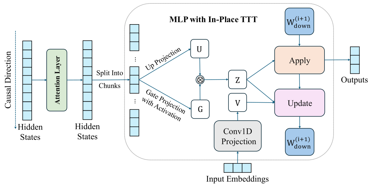
Figure 1 解读：整张 pipeline 图的上半路径是 attention（完全保留原状，不参与 TTT），下半路径是 MLP block，此处被替换为 “MLP with In-Place TTT”。输入序列被切成 chunk（右侧 “Split into chunks”），每个 chunk 经历”Apply 再 Update”的两步循环：

• Apply：用当前 fast weights $W_{\text{down}}^{(i)}$ 处理 chunk $i$ 的中间激活 $Z_{[i]}$，得到该 chunk 的输出；
• Update：基于 $(Z_{[i]},V_{[i]})$ 对 $W_{\text{down}}$ 做一次梯度步，得到 $W_{\text{down}}^{(i+1)}$ 供下一 chunk 使用。

其中 value target $V$ 由 Conv1D & Projection 从 token embedding $X_0$ 中前瞻计算（这是 LM-Aligned Objective 的核心）。在文档边界处 $W_{\text{down}}$ 会被 reset 回预训练值，避免跨文档信息泄漏；ΔW^{(i)} 之间通过 prefix-sum 做并行累加，从而支持 context parallelism。

3.2 复用 MLP 作为 fast weights

Figure 1 解读（放大 MLP 子图）：图中”MLP with In-Place TTT”模块标出三类权重：frozen 的 W_gate、W_up（绿色），以及 dynamic 的 W_down（橙色箭头），体现了”in-place 替换现有 MLP 的 down projection”这一核心设计——没有引入新模块、没有改变总参数量。

Gated MLP 的标准形式：

$$O=(\varphi (H{W}_{\text{gate}}^{\top })\odot (H{W}_{\text{up}}^{\top }))W_{\text{down}}^{\top }$$

作者把 $W_{\text{gate}},W_{\text{up}}$ 视作 frozen slow weights（承载预训练通用知识），把 $W_{\text{down}}$ 视作 fast weights（承载当前 context 的瞬态信息）。选择 $W_{\text{down}}$ 的两个原因：(1) 它是一个大的矩阵（intermediate_size × hidden_size），足以充当高容量的动态 memory；(2) Geva et al. (2020) 揭示 Transformer FFN 本身就在扮演 key-value memory 角色，将其做 in-place 更新在语义上是自然延伸。

Chunk-wise Apply-then-Update。设中间激活 $Z=\varphi (H{W}_{\text{gate}}^{\top })\odot (H{W}_{\text{up}}^{\top })\in {\mathbb{R}}^{n\times d_{ff}}$，value target 与输出 $V,O\in {\mathbb{R}}^{n\times d_{\text{model}}}$。把 $Z,V,O$ 按 chunk size $C$ 切成 $k$ 个 chunk，令 $W_{\text{down}}^{(0)}=W_{\text{down}}$，对每个 chunk $i$：

1. Apply：$O_{[i]}=Z_{[i]}(W_{\text{down}}^{(i)}{)}^{\top }$
2. Update：$W_{\text{down}}^{(i+1)}=W_{\text{down}}^{(i)}-{\lambda }_{\text{lr}}{\nabla }_W\mathcal{L}(Z_{[i]}{W}^{\top },V_{[i]}){|}_{W=W_{\text{down}}^{(i)}}$（${\lambda }_{\text{lr}}$ 即下文 §3.3 / 代码 ttt_lr）

注意：由于 attention 仍然做 token mixing，In-Place TTT 不再需要每 token 更新才能维持 causality，从而允许 C 大到 1024，这是相比 LaCT、Titans 等 TTT-replaces-attention 方案的关键优势。

3.3 LM-Aligned 目标与 closed-form update

Figure 1 解读（放大 LM-Aligned 子图）：Conv1D & Projection 模块从 raw token embedding $X_0$ 中计算 value target $\hat{V}$，其中 Conv1D 做局部 token 的前瞻组合（causal padding），Projection（$W_{\text{target}}$）把组合结果投影到 $d_{\text{model}}$ 空间。这一分支是 In-Place TTT 与常规 reconstruction-TTT 的关键差异。

Target 的设计。常规 TTT 使用 $v_t=W_V{x}_t$（即当前 token 的投影），这让 $W_{\text{down}}$ “记忆自己”，并不能直接贡献 next-token logit。作者把 target 改为：

$$\hat{V}=Conv1D(X_0)W_{\text{target}}\in {\mathbb{R}}^{n\times d_{\text{model}}}$$

其中 $X_0\in {\mathbb{R}}^{n\times d_{\text{model}}}$ 是 token embedding，$Conv1D(\cdot )$ 的 kernel 控制未来若干 token 的局部组合（causal padding 保证 chunk $i$ 的 target 不看 chunk $i$ 以后的数据），$W_{\text{target}}$ 是可学习的投影。极端情况下把 Conv 核设为 [0, 1, 0, …, 0]、$W_{\text{target}}=I$ 即恢复 Next-Token Target；一般情况下近似一个 Multi-Token Prediction（MTP）式的富预测信号。

Loss function：使用 Frobenius inner product（负相似度），

$$\mathcal{L}(Z_{[i]}{W}^{\top },V_{[i]})=-⟨Z_{[i]}{W}^{\top },V_{[i]}{⟩}_F$$

由此导出 closed-form 的梯度更新（论文 Eq. (1)，用 ${\lambda }_{\text{lr}}$ 表示 learning rate，与论文 Theorem 1 记号一致；代码中对应的超参名 ttt_lr 默认值 0.3）：

$$W_{\text{down}}^{(i)}=W_{\text{down}}^{(i-1)}+{\lambda }_{\text{lr}}{\hat{V}}_{[i]}^{\top }{Z}_{[i]}$$

这种形式的更新无需任何额外 Adam/SGD 状态，非常轻量。后续伪代码中的变量 ttt_lr 与此处的 ${\lambda }_{\text{lr}}$ 对应。

Induction head 下的 logit 分析（Theorem 1 简述）。考虑 $(k^{\ast },v^{\ast })$ 出现在位置 $t^{\ast }$，位置 $n>t^{\ast }$ 时查询 $x_n=k^{\ast }$，模型应预测 $x_{n+1}=v^{\ast }$。把前文 chunk 累加的 fast weight delta 写成 $\Delta W_{\text{down}}={\lambda }_{\text{lr}}{\sum }_t{V}_t{Z}_t^{\top }$，于是 query 位置 $n$ 的 logit 变化是

$$\Delta {\ell }_n[w]=E_w^{\top }\Delta W_{\text{down}}{Z}_n$$

• LM-Aligned target：$V_t^{\text{LM}}=E_{x_{t+1}}$。在 embedding 近似正交（$|e_{w_i}^{\top }{e}_{w_j}|\le ϵ$）、key-query 对齐（$\mathbb{E}[z_{t^{\ast }}^{\top }{z}_n]=c_{\text{align}}$）两条标准假设下：

$$\mathbb{E}[\Delta {\ell }_n[v^{\ast }]]\ge {\lambda }_{\text{lr}}{c}_{\text{norm}}^2{c}_{\text{align}}$$ $$|\mathbb{E}[\Delta {\ell }_n[w]]|\le {\lambda }_{\text{lr}}ϵc_{\text{align}},\forall w\ne v^{\ast }$$

• Reconstruction target：$V_t^{\text{rec}}=E_{x_t}$ 只能保证 $|\mathbb{E}[\Delta {\ell }_n[v^{\ast }]]|\le {\lambda }_{\text{lr}}ϵc_{\text{align}}$，无法显著提升 correct token 的 logit。

这给出了 LM-Aligned Objective 有效的清晰理论动机。

3.4 Context-Parallel 实现（chunk-wise 并行扫描）

Figure 1 解读（放大 CP / prefix-sum 子图）：在”Apply & Update”循环右侧画出 $\Delta W^{(i)}$ 的箭头，由 prefix-sum 聚合得到每个 chunk 应用前的 effective $W$。这一 prefix-sum 结构是 In-Place TTT 可以在 Ulysses / Context Parallelism 下保持严格因果的关键。

作者指出更新规则 $\Delta W_{\text{down}}^{(i)}={\hat{V}}_{[i]}^{\top }{Z}_{[i]}$ 具有 associativity，因此可以做 prefix sum 并行化：

1. 对所有 chunk 并行计算 $Z_{[i]},{\hat{V}}_{[i]},\Delta W_{\text{down}}^{(i)}$；
2. 对 $\{\Delta W_{\text{down}}^{(i)}\}$ 做一次 prefix sum 得到累积 $\Delta S_i={\sum }_{j<i}\Delta W_{\text{down}}^{(j)}$；
3. 并行计算每个 chunk 的 effective weight $W_{\text{down}}^{(i-1)}=W_{\text{down}}^{(0)}+{\lambda }_{\text{lr}}\Delta S_i$，以及输出 $O_{[i]}=Z_{[i]}(W_{\text{down}}^{(i-1)}{)}^{\top }$。

因果性的两个细节：(1) 在生成 value target 时 Conv1D 使用 causal padding，保证 chunk $i$ 的 ${\hat{V}}_{[i]}$ 不含 chunk $i$ 之后的信息；(2) 在 document boundary 处把 $W_{\text{down}}$ reset 到预训练初值，避免跨样本信息泄漏。这两点加上 prefix-sum 等价于”严格串行 chunk 更新”，但吞吐上大幅提升。

仓库中的实现用单个 torch.cumsum(dim=chunk_dim) 完成 prefix sum：先把 $\Delta W^{(i)}$ 沿 chunk 轴堆叠为 (B, chunk_num, d_ff, d_model)，并在最前端拼接 $W_{\text{down}}^{(0)}$ 自身作为 “chunk 0 的 effective weight”；cumsum 之后每个位置就是 $W_{\text{down}}^{(i-1)}$。

3.5 Python/PyTorch 伪代码（关键组件）

以下伪代码对应源仓库 hf_models/hf_qwen3/modeling_qwen3.py（训练 / continual-pretrain 路径）与 inference_model/hf_qwen3/modeling_qwen3.py（推理路径）的 Qwen3MLP。

组件 1：TTT-enabled MLP 初始化与 chunk padding

import torch
from einops import rearrange
from transformers.activations import ACT2FN
 
 
class Qwen3MLPTTT(torch.nn.Module):
    """Drop-in TTT-enabled gated MLP (Sec. 3.1).
 
    Mirrors Qwen3MLP.__init__ and Qwen3MLP.padding in hf_models/hf_qwen3/modeling_qwen3.py.
    """
 
    def __init__(self, config, layer_idx=None):
        super().__init__()
        H, F = config.hidden_size, config.intermediate_size
        self.gate_proj = torch.nn.Linear(H, F, bias=False)
        self.up_proj = torch.nn.Linear(H, F, bias=False)
        self.down_proj = torch.nn.Linear(F, H, bias=False)
        self.act_fn = ACT2FN[config.hidden_act]  # e.g. SiLU for Qwen3
        self.layer_idx = -1 if layer_idx is None else layer_idx
 
        if getattr(config, "ttt_mode", False) and self.layer_idx in getattr(
            config, "ttt_layers", []
        ):
            self.ttt_chunk = getattr(config, "ttt_chunk", 8192)
            self.ttt_lr = getattr(config, "ttt_lr", 0.3)
            self.ttt_proj = (
                torch.nn.Linear(H, H, bias=False)
                if getattr(config, "ttt_proj", True) else None
            )
            self.ttt_conv = torch.nn.Conv1d(
                H, H, kernel_size=5, padding=2, groups=H, bias=False,
            )
 
    def padding(self, x):
        """Pad seq-len to a multiple of ttt_chunk, then reshape into chunks."""
        if not hasattr(self, "ttt_chunk"):
            return x
        if x.shape[1] % self.ttt_chunk != 0:
            pad = torch.zeros(
                x.shape[0], self.ttt_chunk - x.shape[1] % self.ttt_chunk, x.shape[2],
                device=x.device, dtype=x.dtype,
            )
            x = torch.cat([x, pad], dim=1)
        return rearrange(x, "b (t c) d -> b t c d", c=self.ttt_chunk)

组件 2：LM-Aligned target 计算（Conv1D + 可选 Projection）

def compute_lm_aligned_target(self, t_chunks: torch.Tensor) -> torch.Tensor:
    """Given chunked hidden states t_chunks (B, T, C, H), return target V_hat with the
    same shape. Mirrors the Conv1D section of Qwen3MLP.forward.
 
    - Conv1d is depthwise (groups=H) with kernel=5, padding=2: local look-ahead.
    - Optional linear projection ttt_proj of shape (H, H).
    - When used inside the cumsum path below, causality is enforced by slicing
      [:, :-1] of (h, t) before contraction, so chunk i only updates W for chunk i+1.
    """
    bs, chunk_num, chunk_size, _ = t_chunks.shape
    t_conv = (
        self.ttt_conv(t_chunks.transpose(-1, -2).reshape(bs * chunk_num, -1, chunk_size))
        .transpose(-1, -2)
        .reshape(bs, chunk_num, chunk_size, -1)
    )
    return t_conv  # ttt_proj applied inside the einsum in 组件 3

组件 3：训练 forward —— chunk-wise 并行扫描（prefix-sum 形式的 CP 实现）

from einops import repeat
from opt_einsum import contract
 
 
def Qwen3MLPTTT_forward(self, x: torch.Tensor, t=None):
    """Training path. Mirrors Qwen3MLP.forward in hf_models/hf_qwen3/modeling_qwen3.py.
 
    Uses cumsum over ΔW chunks to realize the prefix-sum CP formulation in §3.4:
        W^{(i-1)} = W_down + ttt_lr * sum_{j<i} ΔW^{(j)}.
    """
    h = self.act_fn(self.gate_proj(x)) * self.up_proj(x)
    if t is None or not hasattr(self, "ttt_conv"):
        return self.down_proj(h)
 
    t_chunks = self.padding(t)                  # (B, T, C, H)
    h_chunks = self.padding(h)                  # (B, T, C, d_ff)
    bs, chunk_num, chunk_size, _ = t_chunks.shape
 
    t_conv = self.compute_lm_aligned_target(t_chunks)
 
    # ΔW^{(j)} for j = 0 .. T-2  (last chunk never "writes back").
    if self.ttt_proj is not None:
        d_down_proj = contract(
            "b t c h, b t c d, d e -> b t e h",
            h_chunks[:, :-1], t_conv[:, :-1], self.ttt_proj.weight,
        )
    else:
        d_down_proj = contract(
            "b t c h, b t c d -> b t d h",
            h_chunks[:, :-1], t_conv[:, :-1],
        )
 
    # Prepend W_down as the "W^{(0)}" summand so cumsum gives W^{(i-1)} at index i.
    d_down_proj = torch.cat(
        [
            repeat(self.down_proj.weight, "d h -> b 1 d h", b=bs),
            d_down_proj * self.ttt_lr,
        ],
        dim=1,
    )
    d_down_proj_sum = d_down_proj.cumsum(dim=1)     # prefix-sum along chunk axis
 
    down_proj = contract("b t d h, b t c h -> b t c d", d_down_proj_sum, h_chunks)
    return rearrange(down_proj, "b t c d -> b (t c) d")[:, : x.shape[1], :]

组件 4：推理 forward —— Apply-then-Update（顺序更新 fast weight，跨 chunk 携带）

def Qwen3MLPTTT_inference(self, x: torch.Tensor, t=None, past_w=None):
    """Inference path. Mirrors Qwen3MLP.forward in inference_model/hf_qwen3/modeling_qwen3.py.
 
    Returns (output, current_w). The caller is expected to cache current_w across calls
    (e.g. inside TTTDynamicCache) so the fast weight persists over the generation trajectory.
    """
    h = self.act_fn(self.gate_proj(x)) * self.up_proj(x)
    if not hasattr(self, "ttt_conv"):
        return self.down_proj(h)
 
    present_w = self.down_proj.weight.clone() if past_w is None else past_w
    if t is None:
        return torch.nn.functional.linear(h, present_w), present_w
 
    bs, seq_len, _ = x.shape
    if seq_len < self.ttt_chunk:
        return torch.nn.functional.linear(h, present_w), present_w
 
    t_chunks = self.padding(t)
    h_chunks = self.padding(h)
    bs, chunk_num, chunk_size, _ = t_chunks.shape
    t_conv = self.compute_lm_aligned_target(t_chunks)
 
    cur_w = present_w
    y = torch.zeros_like(t_conv)
    # NOTE: inference path in inference_model/hf_qwen3/modeling_qwen3.py only
    # exercises the bs=1 streaming case (KV cache mirrors single-sequence eval),
    # hence the indexing on [0, i] below. For B>1, wrap the inner loop in a
    # for-bsi-in-range(bs) and keep an independent cur_w per batch element.
    for i in range(chunk_num):
        cur_h = h_chunks[0, i]                          # (C, d_ff)
        cur_t = t_conv[0, i]                            # (C, H)
        y[0, i] = contract("d h, c h -> c d", cur_w, cur_h)   # Apply
        # Update: skip ΔW write-back for the last (possibly partial) chunk.
        if seq_len % self.ttt_chunk == 0 or i != chunk_num - 1:
            if self.ttt_proj is not None:
                dw = contract(
                    "c h, c d, d e -> e h",
                    cur_h, cur_t, self.ttt_proj.weight,
                ) * self.ttt_lr
            else:
                dw = contract("c h, c d -> d h", cur_h, cur_t) * self.ttt_lr
            cur_w = cur_w + dw
 
    out = rearrange(y, "b t c d -> b (t c) d")[:, :seq_len, :]
    return out, cur_w

组件 5：Custom weight init for TTT submodules（与 Qwen3PreTrainedModel._init_weights 的 TTT 分支严格对齐）

import torch
import torch.nn as nn
import torch.distributed as dist
 
 
def init_ttt_weights(module: nn.Module, initializer_range: float = 0.02):
    """Mirrors Qwen3PreTrainedModel._init_weights (TTT branch) in
    hf_models/hf_qwen3/modeling_qwen3.py. Applies to:
      - ttt_proj  (nn.Linear, square matrix H x H)  -> zero everywhere, random-normal on diagonal
      - ttt_conv  (nn.Conv1d, kernel=5, groups=H)   -> zero init
    """
    std = initializer_range
 
    if isinstance(module, nn.Linear):
        if module.weight.device.type == "meta":
            return
        # Only square matrices (i.e. ttt_proj, H x H) receive diagonal init; other Linear
        # layers (gate_proj / up_proj / down_proj) are loaded from the pretrained checkpoint.
        if module.weight.shape[0] == module.weight.shape[1]:
            diag_size = module.weight.shape[0]
            weight_data = module.weight.data
 
            if hasattr(weight_data, "_local_tensor"):
                # FSDP2 DTensor: operate on local shard; assume row-sharded.
                local = weight_data._local_tensor
                local.zero_()
                local_rows = local.shape[0]
                num_cols = local.shape[1]
                rank = dist.get_rank()
                start_row = rank * local_rows
 
                g = torch.Generator(device=local.device).manual_seed(42)
                diag_values = torch.randn(
                    diag_size, generator=g, device=local.device, dtype=local.dtype,
                ) * std
 
                local_idx = torch.arange(local_rows, device=local.device)
                global_cols = start_row + local_idx
                mask = global_cols < num_cols
                local_idx = local_idx[mask]
                global_cols = global_cols[mask]
                if len(local_idx) > 0:
                    local[local_idx, global_cols] = diag_values[global_cols]
            else:
                weight_data.zero_()
                diag_values = torch.randn(
                    diag_size, device=weight_data.device, dtype=weight_data.dtype,
                ) * std
                idx = torch.arange(diag_size, device=weight_data.device)
                weight_data[idx, idx] = diag_values
        if module.bias is not None:
            nn.init.zeros_(module.bias)
 
    elif isinstance(module, nn.Conv1d):
        # ttt_conv: zero init so the model starts as vanilla MLP (ΔW ≈ 0 initially).
        module.weight.data.zero_()
        if module.bias is not None:
            module.bias.data.zero_()

关键点：ttt_proj 的对角线初始化为 $\mathcal{N}(0,{\sigma }^2)$（$\sigma =\text{initializer\_range}=0.02$）而非恒等矩阵；非对角线位置严格清零；ttt_conv 完全置零。实现上对 DTensor（FSDP2）做了分片感知：local shard 只写属于自己那部分行的对角元素，全体 rank 共享固定种子 42 以保证跨 rank 一致。ttt_conv 置零可保证训练早期 $\Delta W\approx 0$，TTT 分支从 vanilla MLP 出发逐步学习；ttt_proj 对角线的小幅随机扰动避免了退化解。

Code-to-paper mapping table

Paper Concept	Source File	Key Class / Function	github_ref
In-Place TTT 主体（§3.1，训练 / CP 路径）	hf_models/hf_qwen3/modeling_qwen3.py	Qwen3MLP.__init__、Qwen3MLP.padding、Qwen3MLP.forward(x, t)	ByteDance-Seed/In-Place-TTT@be232482
In-Place TTT 推理（Apply-then-Update，§3.1）	inference_model/hf_qwen3/modeling_qwen3.py	Qwen3MLP.forward(x, t, past_w)（返回 (output, current_w)，由 TTTDynamicCache 跨 step 缓存 fast weight）	ByteDance-Seed/In-Place-TTT@be232482
LM-Aligned target = Conv1D + Projection（§3.3）	hf_models/hf_qwen3/modeling_qwen3.py	self.ttt_conv（depthwise Conv1d, kernel_size=5, padding=2, groups=H, bias=False）+ self.ttt_proj（Linear H→H，可通过 config.ttt_proj=False 关闭）	ByteDance-Seed/In-Place-TTT@be232482
Chunk-wise prefix-sum parallel scan（§3.4）	hf_models/hf_qwen3/modeling_qwen3.py	Qwen3MLP.forward 中的 d_down_proj.cumsum(dim=1) 段，对应 $W_{\text{down}}^{(0)}+{\lambda }_{\text{lr}}{\sum }_{j<i}\Delta W^{(j)}$ 的 prefix sum	ByteDance-Seed/In-Place-TTT@be232482
TTT 子模块权重初始化（对角随机 + 零 Conv，DTensor-aware）	hf_models/hf_qwen3/modeling_qwen3.py	Qwen3PreTrainedModel._init_weights（nn.Linear square-matrix 分支：local-shard zero + 对角 randn(..) * 0.02，固定 seed=42；nn.Conv1d 分支：全零）	ByteDance-Seed/In-Place-TTT@be232482
Decoder layer（默认把 hidden_states 同时作为 target）	hf_models/hf_qwen3/modeling_qwen3.py	Qwen3DecoderLayer.forward：if target_states is None and self.is_ttt_layer: target_states = hidden_states; hidden_states = self.mlp(hidden_states, t=target_states)	ByteDance-Seed/In-Place-TTT@be232482
TTT 作用于哪些 layer 的配置	hf_models/hf_qwen3/configuration_qwen3.py	ttt_mode、ttt_layers、ttt_chunk、ttt_lr、ttt_proj	ByteDance-Seed/In-Place-TTT@be232482
Qwen3-4B-Base 的 continual pretrain 配置	configs/pretrain/qwen3_longct.yaml	ttt_layers=[0,6,12,18,24,30,36], ttt_mode=true, ttt_proj=true, ttt_lr=3, ttt_chunk=4096	ByteDance-Seed/In-Place-TTT@be232482
LLaMA-3.1-8B 同步版本	configs/pretrain/llama3_longct.yaml、hf_models/hf_llama/*	LlamaMLP（与 Qwen3MLP 对称实现）	ByteDance-Seed/In-Place-TTT@be232482
Train entry	tasks/train_torch.py、train.sh	—	ByteDance-Seed/In-Place-TTT@be232482
Infer entry	tasks/infer.py、eval.sh	—	ByteDance-Seed/In-Place-TTT@be232482
RULER 4k~256k benchmark 配置	eval_config/ruler_*.py	—	ByteDance-Seed/In-Place-TTT@be232482
DCP → HF checkpoint 合并	scripts/merge_dcp_to_hf.py	—	ByteDance-Seed/In-Place-TTT@be232482

4. Experimental Setup (实验设置)

作者围绕三个研究问题设计实验（Sec. 4）：

Q1：In-Place TTT 作为 drop-in 增强预训练 LLM 的效果？ Q2：从零训练时，与现有 TTT / 线性 / SWA 方案相比的优劣？ Q3：关键设计（state size、chunk size、LM-aligned objective）各自的贡献？

Q1：Drop-in enhancement on pretrained LLMs

• 主实验：Qwen3-4B-Base（原生 32k 上下文）；
• 两阶段 continual training：Stage 1 约 20B tokens @ 32k context，Stage 2 约 15B tokens @ 128k context；
• 用 YaRN 对 RoPE 做 scale 以支持长上下文；
• Baseline 与 In-Place TTT 使用完全相同的 curriculum、只切换是否启用 TTT；
• 评测：RULER 4k~256k（OpenCompass），256k 专门检验 extrapolation；
• 扩展实验：同协议应用到 LLaMA-3.1-8B 和 Qwen3-14B-Base（额外加入 64k + YaRN 组）。

Q2：From-scratch pre-training

• 500M / 1.5B 比较对象：Transformer + SWA、GLA、DeltaNet、LaCT（SWA 底）、In-Place TTT（SWA 底）；
• 32k sequence length、TogetherAI 数据；
• 主指标：Sliding Window Perplexity（固定末尾 block、延长前缀）on Pile + Proof-Pile-2；
• 4B 比较对象：Full-Attn vs. Full-Attn + In-Place TTT，SWA vs. SWA + In-Place TTT，120B tokens @ 8k 预训练；
• 评测：HellaSwag / ARC-E / ARC-C / MMLU / PIQA 常识推理 + RULER 4k/8k/16k。

Q3：Ablation

• 模型：1.7B、RULER benchmark；
• 扫描维度：state size（TTT 层数，0.5× / 1× / 4× baseline state size）、chunk size（256 / 512 / 1024 / 2048）、LM-Aligned 目标（w Conv, Proj / w/o Conv / w/o Proj / w/o Conv, Proj）。

默认超参：

• 论文 §4.3 推荐配置：ttt_chunk=1024（兼顾效率与精度，C=512 / C=1024 同档最优），代码层面 getattr(config, "ttt_chunk", 8192) 提供保守 fallback；
• configs/pretrain/qwen3_longct.yaml（Qwen3-4B-Base 实际使用）：ttt_layers=[0, 6, 12, 18, 24, 30, 36]、ttt_mode=true、ttt_proj=true、ttt_lr=3、ttt_chunk=4096；
• ttt_proj：square Linear H→H，按 Qwen3PreTrainedModel._init_weights 对角随机初始化 $\mathcal{N}(0,{\sigma }^2)$（$\sigma =0.02$），非对角清零；并非恒等矩阵；
• ttt_conv：groups=H 的 5-tap depthwise Conv1d（kernel_size=5, padding=2），权重 zero-init，使训练初期 $\Delta W\approx 0$；
• continual training 使用 FSDP2 + Context Parallelism + flash attention。

5. Experimental Results (实验结果)

5.1 RULER 主表（Qwen3-4B-Base）

Model	4k	8k	16k	32k	64k	128k	256k
Mistral-7B	93.6	91.2	87.2	75.4	49.0	13.8	–
GLM3-6B	87.8	83.4	78.6	69.9	56.0	42.0	–
Phi3-medium-14B	93.3	93.2	91.1	86.8	78.6	46.1	–
Llama3-8B	92.8	90.3	85.7	79.9	76.3	69.5	–
Qwen3-4B (Instruct)	95.1	93.6	91.0	87.8	77.8	66.0	–
Baseline (Qwen3-4B-Base + continual training)	96.6	94.1	92.1	88.7	74.3	74.8	41.7
+ In-Place TTT	96.1	95.6	92.7	89.3	78.7	77.0	43.9

核心现象：

• 在 4k 上略低 0.5pp（有限噪声），在 8k 起的所有长度上稳定胜出 baseline；
• 64k / 128k / 256k 分别 +4.4 / +2.2 / +2.2 pp，即越长越有效；
• 256k 是 extrapolation 区（训练最长到 128k），In-Place TTT 仍保持增益，表明其确实在”压缩 context 信息”而不是简单记忆位置模式。

扩展：LLaMA-3.1-8B / Qwen3-14B-Base（Tab. 2）

Base Model	Method	4k	8k	16k	32k	64k	64k+YaRN
LLaMA-3.1-8B	Baseline	93.9	92.1	92.5	91.1	81.6	–
LLaMA-3.1-8B	+ In-Place TTT	94.4	93.0	93.3	91.7	83.7	–
Qwen3-14B-Base	Baseline	96.8	95.0	94.6	90.7	67.9	81.3
Qwen3-14B-Base	+ In-Place TTT	97.2	95.7	95.2	91.2	70.6	82.5

• 不同模型家族（LLaMA vs. Qwen3）、不同规模（4B/8B/14B）均保持一致正收益；
• 与 RoPE-scale 技术（YaRN）正交，可叠加使用。

5.2 From-scratch 比较：500M / 1.5B perplexity

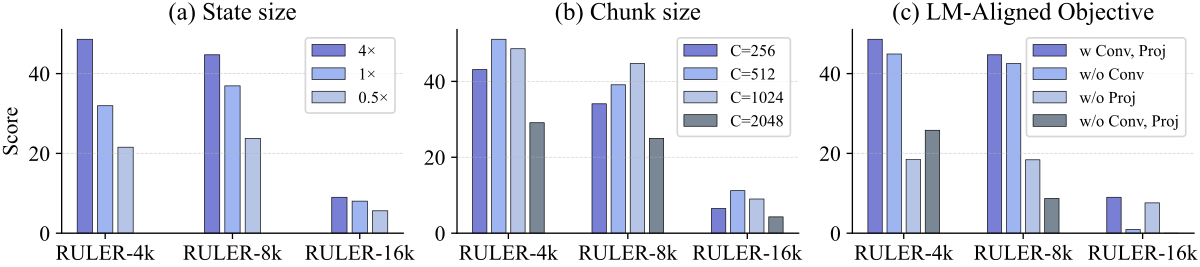
Figure 2 解读：两张图分别展示 500M / 1.5B 模型在 Pile 验证集上的 Sliding Window Perplexity 曲线。x 轴 context length（2k~32k），y 轴 PPL。

• 500M：SWA、GLA、DeltaNet 的 PPL 在 8k 之后都明显回升，LaCT 稍好但仍呈上翘趋势；In-Place TTT 唯一保持单调下降，说明它是唯一能有效压缩长上下文信息的架构。
• 1.5B：所有方案绝对 PPL 更低；In-Place TTT 仍然稳定领先约 0.1~0.3 PPL。

5.3 From-scratch 4B 表（Tab. 3）

Model	Architecture	HellaSwag	ARC-E	ARC-C	MMLU	PIQA	RULER-4k	RULER-8k	RULER-16k
Baseline	Full Attn.	55.67	64.52	33.19	36.43	72.63	45.77	38.09	6.58
Baseline	SWA	54.92	64.18	32.85	36.06	72.58	14.77	9.91	5.07
I.P. TTT	Full Attn.	55.85	64.98	32.34	37.42	73.29	49.98	43.82	19.99
I.P. TTT	SWA	55.24	64.60	33.70	36.48	72.03	28.33	26.80	7.57

关键结论：

• 常识推理基本全面提升（HellaSwag / ARC-E / MMLU / PIQA 均更高）；
• Long-context 提升最为显著：RULER-16k 下 Full-Attn+TTT 从 6.58 → 19.99（3× gain），SWA+TTT 从 9.91 → 26.80（2.7× gain），证明 In-Place TTT 的核心价值在 long-context 压缩而非 short context。

5.4 Ablation：state size / chunk size / objective

State size（Figure 3(a)）：按 TTT-enabled layer 数控制 state 大小（0.5× / 1× / 4×）。结果 4× > 1× > 0.5×，即更多 TTT 层→ 更大 fast-weight state → 更强 long-context。这说明复用 MLP state 的方向是对的，还有进一步 scale 的空间。

Chunk size（Figure 3(b)）：C ∈ {256, 512, 1024, 2048}。结果 512 / 1024 最优；256 过细、2048 过粗。验证”In-Place TTT 天然支持大 chunk”（这是它与 LaCT 等 TTT-as-attention 方案的关键差异）。C=1024 在精度相近前提下吞吐最高，被选作默认。

LM-Aligned objective（Figure 3(c)）：

Variant	RULER-4k	RULER-8k	RULER-16k
w Conv, Proj（默认）	最高	最高	最高
w/o Conv（仅 Proj）	明显下降	显著下降	显著下降
w/o Proj（仅 Conv）	小幅下降	小幅下降	中等下降
w/o Conv, Proj（reconstruction）	最低	最低	最低

Conv 在长上下文上决定性地重要（让 target 包含未来 token 信息），Projection 在短上下文上更关键（灵活表达映射）。二者都去掉即退化成 reconstruction target，全面变差。这与 Theorem 1 的预测完全吻合。

5.5 效率

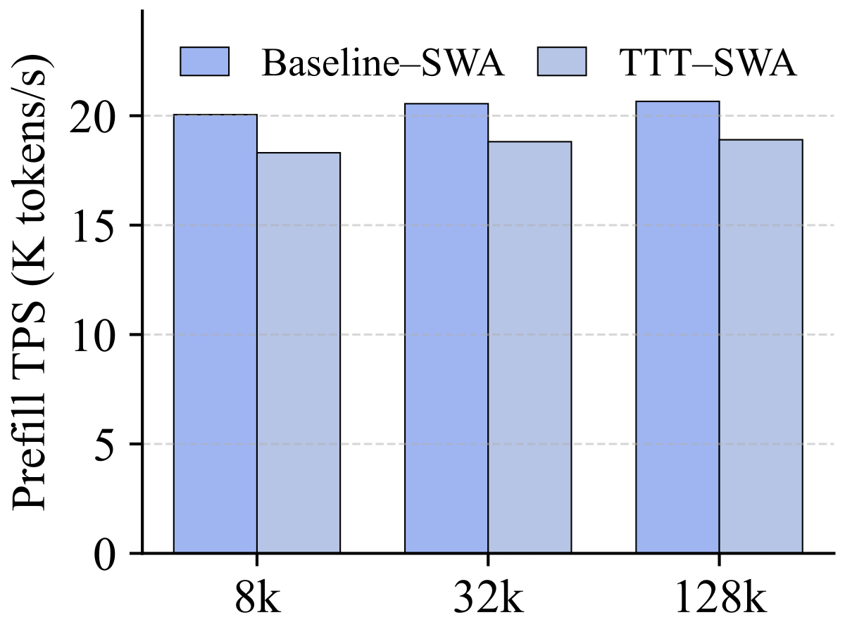
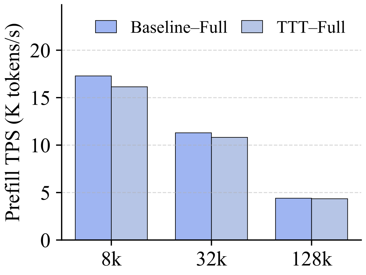
Figure 4(a-b) 解读：分别是 SWA 底与 Full-Attn 底下的 prefill throughput（K tokens/s，越高越好）。x 轴 context length（8k / 32k / 128k）。Baseline vs. TTT 曲线几乎重合，最大差距约 5~8%，说明 In-Place TTT 对推理吞吐几乎不增加开销。

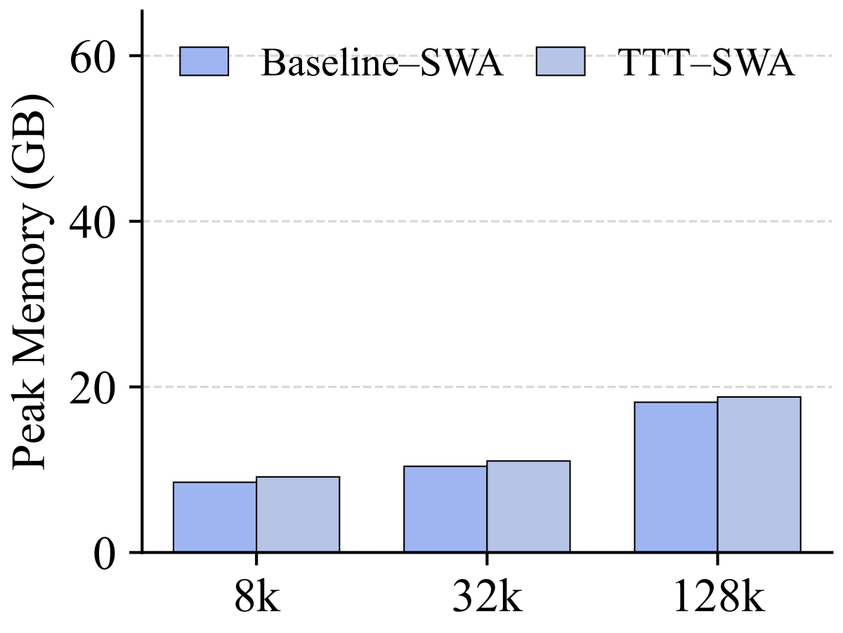
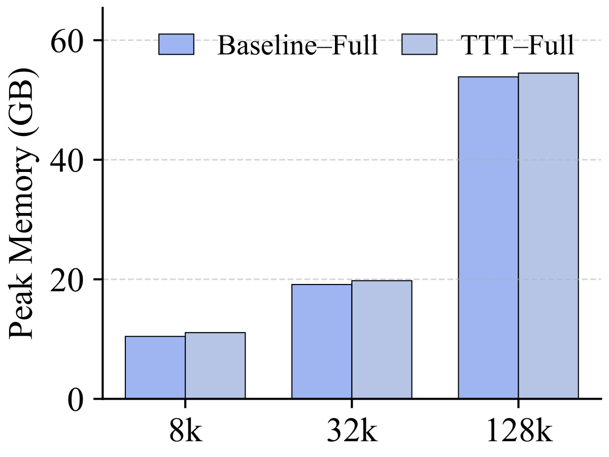
Figure 4(c-d) 解读：Peak memory (GB)。TTT 版本的内存占用与 Baseline 基本一致——因为 fast weight 与 MLP 原有权重共享 slot，额外只存一个 clone、Conv1D 与 Proj 几兆参数。这再次强化”drop-in”承诺：不需要额外硬件或大幅重训。

5.6 Sanity-check：TTT results 细节

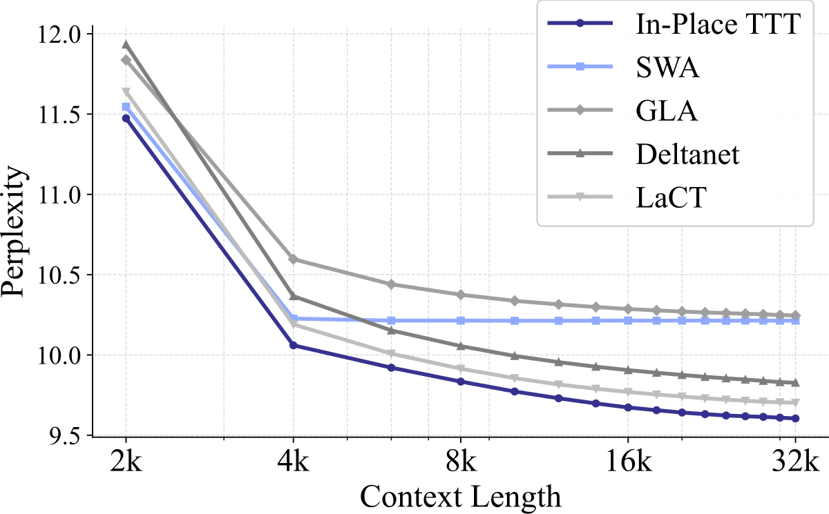
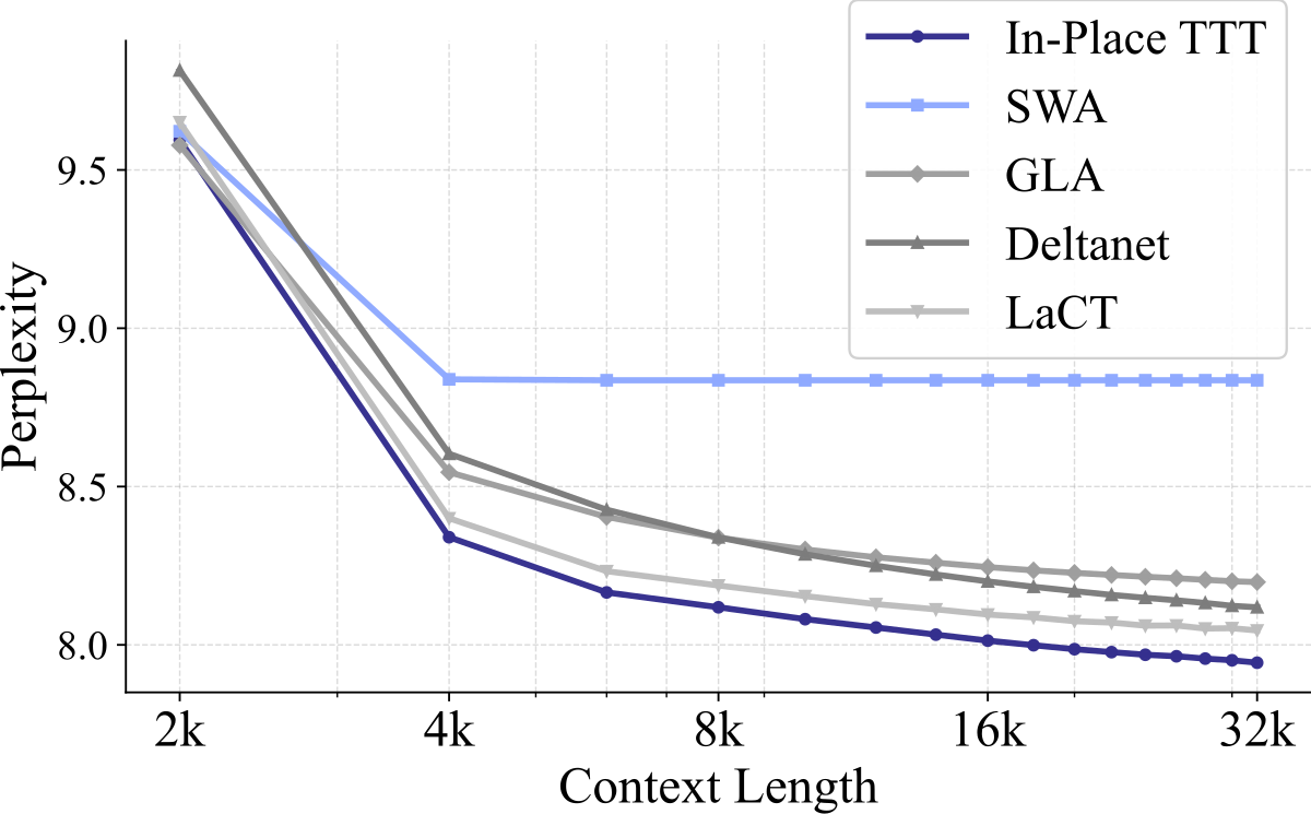
Figure 扩展解读：对 500M / 1.5B 模型做 Sliding Window PPL（y 轴）随 context length（x 轴）变化的放大图，可看到 In-Place TTT 的曲线相对 baseline 系列在 8k→32k 区间有单调分离的下降斜率，而 SWA/GLA/DeltaNet/LaCT 会在某个长度后停止下降甚至回升。这一”长度越长收益越大”的趋势与 Table 1 的 4B 结果一致。

5.7 Discussion & 局限

• 结论：In-Place TTT 提供了一条不破坏预训练权重、兼容 context parallelism、具有 LM-aligned 理论保证的 fast-weights 实现路径。它让 Qwen3-4B 这种既有模型以 35B tokens 的 continual training 就能把 128k RULER 提升约 +2.2 pp，是目前对现有 LLM 最友好的 TTT 方案之一。
• 推广：该框架可以自然地叠加到 Full-Attn、SWA、GLA、DeltaNet 等多种 backbone，以及 YaRN、NTK-scaling 等 RoPE 扩展方法。
• 局限：
  • LM-aligned objective 的理论证明在 induction-head 单层简化场景下给出，未覆盖多层复杂 circuit；
  • 当前只实例化了 down_proj 的更新，其他 MLP 项（gate/up）或 attention 投影能否同样重新用于 TTT 未展开；
  • Chunk size、state size、lr 等仍然需要按模型规模调节，缺少 auto-tune；
  • 依赖 YaRN 做 RoPE scale；极端超长（>256k）行为有待继续 scale 数据与训练。