Adam’s Law: Textual Frequency Law on Large Language Models

Paper: arXiv:2604.02176 Code: HongyuanLuke/frequencylaw Code reference: main @ 515c88ec (2026-04-14)

1. Motivation (研究动机)

这篇论文要回答一个被 prompt engineering 和数据筛选长期绕开的具体问题：当两个输入是同义 paraphrase、但表达方式的文本频率不同，LLM 更应该看到哪一个？已有工作已经知道 prompt wording 会显著改变输出质量，也知道数据质量、数据量、课程学习顺序会影响训练；但它们通常没有把“同义语义下的文本频率”作为一个可测量变量来研究。

作者的核心假设是：高频表达更接近预训练分布，模型在预训练中见过相似 token/phrase 的概率更高，因此更容易“读懂”并稳定地执行下游任务；低频表达可能包含更复杂、更少见的词汇或结构，语义虽然相同，但会让模型落到更不熟悉的输入区域。这个问题值得研究，因为它同时影响两类常见场景：推理时的 prompt paraphrasing（零训练成本）和 LoRA/SFT 时有限训练预算下的数据选择与排序。

论文因此提出一个 frequency-centric 框架：先定义 Textual Frequency Law (TFL)，再用 Textual Frequency Distillation (TFD) 改善闭源模型训练语料不可见时的频率估计，最后用 Curriculum Textual Frequency Training (CTFT) 把频率从“选择哪个 paraphrase”扩展到“训练样本按什么顺序喂给模型”。

2. Idea (核心思想)

核心 insight：在语义保持不变时，文本频率不是表面风格特征，而是模型熟悉度的代理变量；高频 paraphrase 通常让模型获得更低输入 NLL、更稳定的表示与更好的任务输出。它和传统 “easy-to-hard” curriculum 的差别是，TFL 不直接用句法复杂度或长度定义难度，而是用语料频率估计模型对表达方式的熟悉程度。

方法上，论文把一个输入 $x$ 扩展成多个同义 paraphrase 集合 $P$ ，为每个候选估计 sentence-level frequency，然后选择更高频的候选用于 prompting 或 fine-tuning。由于实际 LLM 训练语料往往不可得，论文先用开放在线资源估计频率，再让目标 LLM 对数据做 story completion 生成 $D^{'}$ ，用这批“模型自己会延展出的语料”调整频率估计。

与 synonym replacement、普通 paraphrase augmentation 或传统 curriculum learning 相比，TFL/TFD/CTFT 的根本区别是：它不是随机替换、更不是把所有 paraphrase 都混进训练；它先把同义表达按频率排序，并在推理和训练中显式偏向高频表达，同时在训练顺序上利用低频到高频的 curriculum。

3. Method (方法)

3.1 总体框架

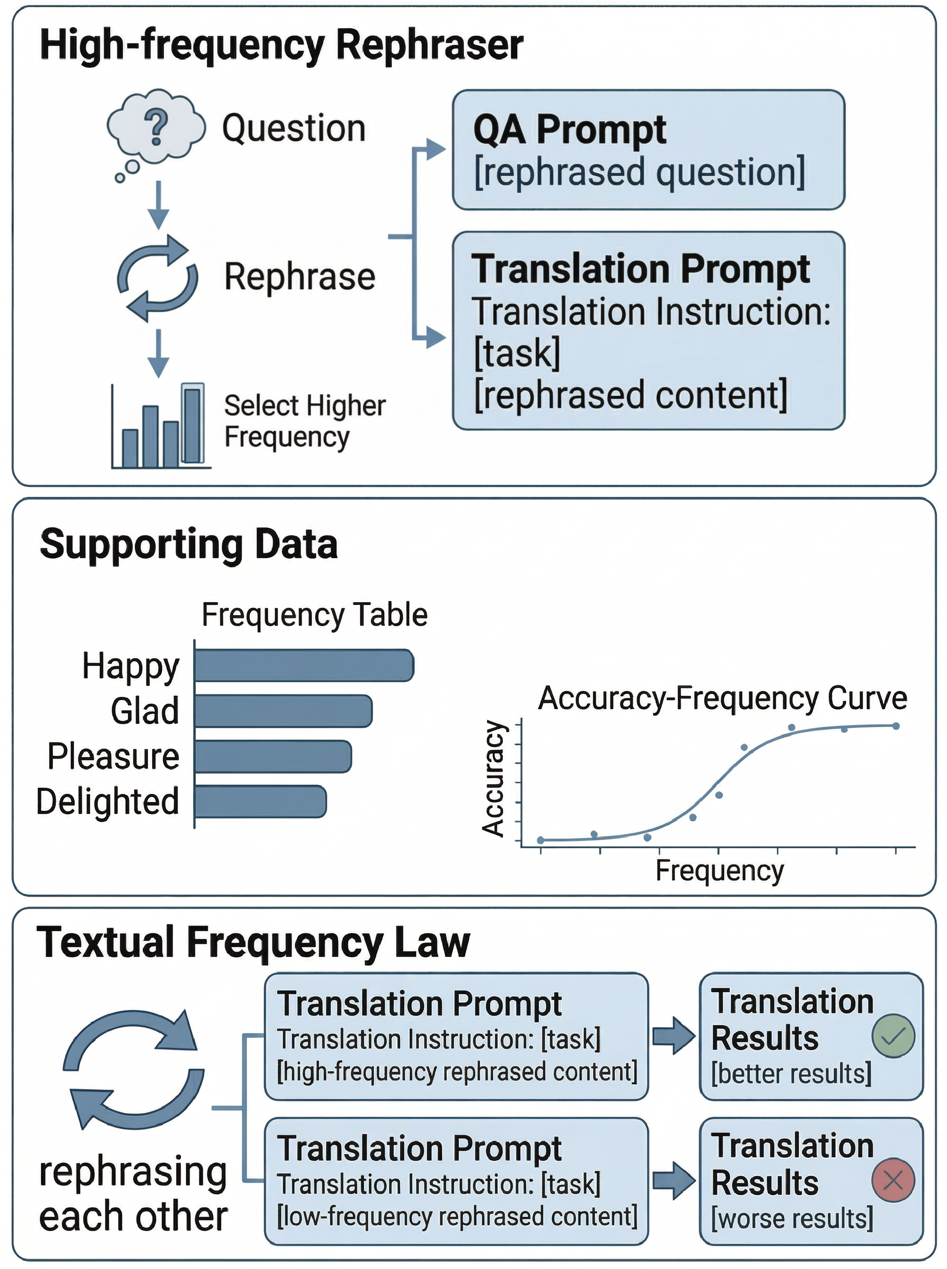
Figure 1 解读：上半部分展示 High-frequency Rephraser：原始 question/input 先被 paraphrase，再从候选表达中选择更高频版本，最后拼入 QA prompt 或 translation prompt。中间部分说明频率来自词级 frequency table 的句级估计；下半部分给出直觉：同义 translation prompt 中，高频版本更容易得到正确 translation results，低频版本更容易失败。

直觉上，这个框架把“模型是否熟悉输入表达”从不可观测变量转成可操作的频率分数。对 prompting，它只改写输入，不改模型；对 fine-tuning，它把同义输入和原始标签配对，让模型在有限 LoRA/SFT 预算内优先学习更贴近预训练分布的表达；对 CTFT，它又利用低频表达的多样性，先训练低频再过渡到高频，使模型既看到困难/多样表达，又最终对高频表达形成稳定映射。

3.2 任务形式化与 TFL

LLM 被写成 instruction + input 到 output 的 autoregressive Seq2Seq：

P (y ∣ i, x) = j = 1 \prod T P (y_{j} ∣ y_{1}, \dots, y_{j - 1}, i, x) .

论文把 instruction 和 actual input 合并记作 $x$ 。给定同义 paraphrase 集合 $P$ ，TFL 选择句级频率最高的表达：

argmax_{x \in P} (sfreq (x, D)) .

句级频率由词级频率估计。论文正文写为：

sfreq (x, D) = K \frac{1}{\prod _{k = 1}^{K} wfreq ( x _{k} , D )} .

论文公式与 released code 实现差异：正文一方面说选择 argmax sfreq，另一方面公式和代码都把分数写成“词频倒数的几何/乘积型分数”；在 released code 中，frequency.py 会把最大 inverse-frequency score 写入 *_lowfrequency.txt，把最小 inverse-frequency score 写入 *_highfrequency.txt，即代码实际语义是“score 越小越高频”。因此阅读公式时要把 $sfreq$ 理解为论文命名上的 frequency score，而复现实验时要遵循代码的 min/max 方向；这是一个需要显式记录的 paper-vs-code gap。

3.3 TFD：用目标 LLM 生成语料修正频率估计

TFD 的动机是：闭源 LLM 的真实训练语料不可见，开放资源只能给出近似频率。论文让 LLM 对现有文本做 story completion：

Please conduct story completion on the following data: <textual data>

生成语料记为 $D^{'}$ ，并从中得到第二个频率估计：

F_{2} = sfreq (x, D^{'}) .

设开放资源估计为 $F_{1}$ ，最终频率为：

F (x) = α F_{1} (x) + (1 + ζ \mathbbm 1 (F_{1} (x) = 0)) β F_{2} (x) .

其中 $ζ$ 是 strengthening factor：当开放语料中某些词频几乎为 0 时，提高 distilled frequency 的作用。released code 里的 newfrequency.py 使用 Brown corpus 与 your_new_generate_file.txt 生成的新语料，先对新旧概率做 scale/align，再把概率合并；MT-SFT/sort_frequency.py 进一步用 unigram/bigram 混合频率（默认 UNIGRAM_WEIGHT=0.6, BIGRAM_WEIGHT=0.4, ALPHA=0.15）计算 sentence score。

3.4 CTFT：频率 curriculum

CTFT 将普通训练集 $T$ 中每个样本按频率排序：

sort_{x_{n} \in T} (F (x_{n})), n = 1, \dots, N .

论文定义的训练顺序是从低 sentence-level frequency 到高 sentence-level frequency。直觉是：低频表达更复杂、更多样，先训练可以让模型覆盖困难输入；随后过渡到高频表达，最终让模型在更熟悉、更稳定的输入分布上收敛。released code 的 MT-SFT/sort_frequency.py 是 CTFT 数据排序的实现入口，但 as released 版本存在一个复现风险：第 153 行引用了未定义变量 freq_dict_low，且输出文件名 *_highTolow_all.json 与论文 “low-to-high” 描述需要人工核对。

3.5 TFPD 数据构造

论文构建 Textual Frequency Paired Dataset (TFPD)：用 GPT-4o-mini 对 GSM8K、FLORES-200、CommonsenseQA 等数据生成高频/低频 paraphrase，随后由 3 名英语语言学相关背景标注者检查原句、高频句、低频句是否同义；只有 3 人都认为语义一致的样本被保留。论文正文给出的最终数据规模是：GSM8K 从 1,319 个 test instances 中保留 738 对，FLORES-200 从 1,012 个 dev-test instances 中保留 526 对；表格还列出 CR 为 575 对、TC 为 114 对。

3.6 理论证明要点

附录证明把 TFL 写成“频率更高的 paraphrase 倾向于更低 NLL”。Token-level 假设采用 Zipf law：

P (w_{r}) = \frac{r ^{- s}}{Z}, s > 0, Z = n = 1 \sum ∣ V ∣ n^{- s} .

理想 self-information 为：

- ln P (w_{r}) = s ln r + ln Z = s ln r + C .

如果模型 marginal probability 与真实 marginal probability 的 log-domain 误差满足 $∣ ln Q_{θ} (w_{r}) - ln P (w_{r}) ∣ \leq ε (r)$ ，则 marginal token NLL 满足：

ℓ_{θ}^{m} (w_{r}) = s ln r + C + δ_{w_{r}}, ∣ δ_{w_{r}} ∣ \leq ε (r) .

句级损失分解为：

ℓ_{θ} (x) = - ln sfreq (x) + \overset{ˉ}{δ}_{x} + \overset{η}{ˉ}_{x},

其中 $\overset{ˉ}{δ}_{x}$ 是 marginal approximation error， $\overset{η}{ˉ}_{x}$ 是 marginal-to-conditional contextual discrepancy。对两个同义句 $x, x^{'}$ ，若 $sfreq (x) > sfreq (x^{'})$ ，一个充分条件是：

ln \frac{sfreq ( x )}{sfreq ( x ^{'} )} > (\overset{ε}{ˉ}_{x} + η_{x}) + (\overset{ε}{ˉ}_{x^{'}} + η_{x^{'}}),

则 $ℓ_{θ} (x) < ℓ_{θ} (x^{'})$ 。作者也明确说明：从低 NLL 到更好 task performance 不是严格 theorem，而是由实验支持的经验假设。

3.7 Released code 对应关系

Code reference: main @ 515c88ec (2026-04-14) — pseudocode and mapping based on this commit

Paper Concept	Source File	Key Class/Function
TFL 词频/句频打分	`frequency.py`, `newfrequency.py`	`clean_and_tokenize`, `compute_zipf_frequency`, `compute_sentence_score`
高频/低频 paraphrase 生成	`rephrase.py`	`process_questions`, `process_file`
TFD 新语料合并	`newfrequency.py`, `MT-SFT/sort_frequency.py`	`load_and_normalize_corpus`, `align_and_merge`, `get_ngram_frequencies`
TFPD 数据集	`datasets/*.txt`, `issame.py`	高频/低频文本文件；语义一致性检查脚本
Math Reasoning 推理	`reply_mr.py`, `get_correct_answer.py`, `judge.py`	GPT-style 请求、答案数字提取、正确性判断
Machine Translation 推理	`reply_mt.py`, `MT-SFT/runmodel.py`	翻译 prompt、LoRA adapter 推理、生成翻译输出
CTFT 数据排序	`MT-SFT/sort_frequency.py`, `MT-SFT/merge.py`	`calculate_weighted_score_new`, `main`, JSON 数据合并

实现导向伪代码如下，保留 released code 的关键方向与复现风险：

from collections import Counter, defaultdict
import math
import re
import numpy as np
 
STOP_WORDS = set()
MIN_FREQ = 1
UNIGRAM_WEIGHT = 0.6
BIGRAM_WEIGHT = 0.4
ALPHA = 0.15
 
def clean_and_tokenize(text: str, remove_stopwords: bool = True) -> list[str]:
    text = re.sub(r"[^a-zA-Z'-]", " ", text.lower())
    text = re.sub(r"(?<!\w)['-]|['-](?!\w)", "", text)
    words = re.sub(r"\s+", " ", text).strip().split()
    expanded = []
    for word in words:
        expanded.extend([w for w in word.split("-") if w] if "-" in word else [word])
    return [w for w in expanded if (not remove_stopwords or w not in STOP_WORDS)]
 
 
def inverse_frequency_score(sentence: str, word_counts: Counter) -> float:
    # frequency.py: smaller score means more frequent in released file naming.
    words = clean_and_tokenize(sentence)
    if not words:
        return 0.0
    inv_freqs = [1.0 / word_counts.get(w, 1) for w in words]
    return float(np.prod(inv_freqs) / len(words))
 
 
def split_high_low_paraphrases(paraphrases: list[str], word_counts: Counter) -> tuple[str, str]:
    scored = [(s, inverse_frequency_score(s, word_counts)) for s in paraphrases]
    scored.sort(key=lambda x: x[1])
    high_frequency = next(s for s, _ in scored if len(s) >= 10)       # min inverse score
    low_frequency = next(s for s, _ in reversed(scored) if len(s) >= 10)  # max inverse score
    return high_frequency, low_frequency

def align_and_merge_probabilities(old_probs: dict[str, float], new_probs: dict[str, float], eps: float = 1e-8) -> dict[str, float]:
    # newfrequency.py: align model-distilled corpus scale to Brown/open-resource corpus.
    common = {w for w in old_probs if w in new_probs and old_probs[w] > 1e-10 and new_probs[w] > 1e-10}
    gamma = np.median([(old_probs[w] + eps) / (new_probs[w] + eps) for w in common]) if len(common) > 10 else 1.0
    merged = {}
    for word in set(old_probs) | set(new_probs):
        p_old = old_probs.get(word, eps)
        p_new = new_probs.get(word, eps) * gamma
        merged[word] = p_old * p_new  # released code uses product, not beta-weighted sum.
    total = sum(merged.values()) or 1.0
    return {w: p / total for w, p in merged.items()}
 
 
def tfd_sentence_score(sentence: str, probs: dict[str, float], eps: float = 1e-8) -> float:
    words = clean_and_tokenize(sentence)
    if not words:
        return 0.0
    return float(np.exp(np.mean(np.log([1.0 / probs.get(w, eps) for w in words]))))

def weighted_ngram_score(sentence: str, freq_dict: dict) -> float:
    # MT-SFT/sort_frequency.py: larger combined score means higher observed unigram/bigram frequency.
    words = clean_and_tokenize(sentence)
    bigrams = list(zip(words, words[1:]))
    uni = [freq_dict["unigram"].get(w, MIN_FREQ) for w in words]
    bi = [freq_dict["bigram"].get(b, MIN_FREQ) for b in bigrams] or [MIN_FREQ]
    uni_score = math.exp(sum(math.log(x) for x in uni) / len(uni)) if uni else MIN_FREQ
    bi_score = math.exp(sum(math.log(x) for x in bi) / len(bi))
    return (uni_score ** UNIGRAM_WEIGHT) * (bi_score ** BIGRAM_WEIGHT)
 
 
def build_ctft_epoch(entries: list[dict], freq_dict: dict) -> list[dict]:
    # Paper CTFT: train from lower sentence-level frequency to higher frequency.
    # As released, sort_frequency.py has an undefined freq_dict_low variable near final sorting,
    # so this is the intended low-to-high curriculum rather than a guaranteed runnable script path.
    return sorted(entries, key=lambda e: weighted_ngram_score(e["input"], freq_dict))

4. Experimental Setup (实验设置)

4.1 数据集与任务

论文覆盖四类任务：Math Reasoning (MR)、Machine Translation (MT)、Commonsense Reasoning (CR)、Tool Calling (TC)。TFPD 表格给出的 paired data 规模为：MR 738 对、MT 526 对、CR 575 对、TC 114 对；正文还说明 GSM8K 从 1,319 个原始 test instances 保留 738 对，FLORES-200 从 1,012 个 dev-test instances 保留 526 对。MT prompting 随机选取 FLORES-200 的 100 种语言，其中按 Joshi et al. 语言资源分类，class 0/1 合计 62 种（16 + 46），超过一半是低资源语言；CTFT fine-tuning 只使用 Kabuverdianu (kea_Latn)、Kikuyu (kik_Latn)、Pangasinan (pag_Latn) 和 Standard Latvian (lvs_Latn)。

4.2 Baselines 与模型

Prompting 实验使用 GPT-4o-mini、DeepSeek-V3、doubao-1.5-pro-32k、qwen2.5-7b-instruct、Llama-3.3-70B-Instruct 等模型；DeepSeek-V3 被描述为 671B MoE。Fine-tuning 实验全部在 qwen2.5-7b-instruct 上进行，采用 LoRA fine-tuning。对比包含 low-frequency partition、high-frequency partition、synonym replacement baseline、原始 FLORES-200 fine-tuned model、easy-to-hard curriculum（Max Dependency Tree Depth）、high-to-low baseline、只用 LF/HF 或 1/2 LF + 1/2 HF 的 fine-tuning 组合。

4.3 指标

MR 与 CR 使用 accuracy；MT 使用 sacreBLEU 的 chrF 和 BLEU，并使用 COMET wmt22-comet-da 做 neural evaluation。论文给出 chrF 参数 nworder=6, ncorder=6, beta=2，BLEU 使用 ngram=4、权重 (0.25,0.25,0.25,0.25)、method1 smoothing、nltk_word_tokenize tokenizer。COMET 只支持 37/100 种语言。

4.4 Fine-tuning 配置

论文附录 Table np 给出的 fine-tuning 超参为：quantization_bit=4，stage=sft，do_train=true，finetuning_type=lora，lora_target=all，template=qwen，cutoff_len=1024，max_samples=3000，overwrite_cache=true，preprocessing_num_workers=16，logging_steps=10，save_steps=500，per_device_train_batch_size=1，gradient_accumulation_steps=8，learning_rate=1.0e-4，num_train_epochs=10.0，lr_scheduler_type=cosine，warmup_ratio=0.1，bf16=true。

Released code 中没有对应的完整 LLaMA-Factory/YAML launch config，也没有 GPU type/count；MT-SFT/runmodel.py 只给出推理配置：BASE_MODEL_PATH="Qwen2.5-7B-Instruct"，LoRA adapter path 示例为 ./saves/qwen-7b/lora/sft_kea_Latn_hightolow，max_length=2048，max_new_tokens=512，temperature=0.7，top_p=0.9，repetition_penalty=1.2，do_sample=True。因此硬件配置与完整训练命令属于“论文未详细说明 / released code 未提供”。

5. Experimental Results (实验结果)

5.1 Prompting：Math Reasoning

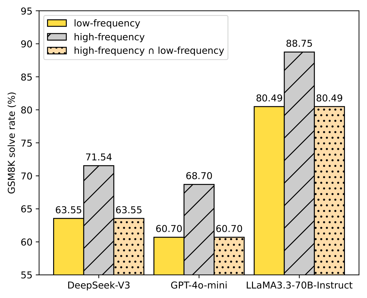
Figure 2 解读：GSM8K 上，高频 paraphrase 在三个模型上都提升 solve rate：DeepSeek-V3 从 63.55% 到 71.54%，GPT-4o-mini 从 60.70% 到 68.70%，Llama-3.3-70B-Instruct 从 80.49% 到 88.75%。图中的 “high-frequency ∩ low-frequency” 与 low-frequency 数值相同，说明作者观察到：低频版本已经做对的样本，高频版本也保持正确；高频主要修复原本低频做错的样本。

附录模型尺度实验显示，qwen-2.5 从 0.5B 到 72B 均满足 high > low：0.5B 为 0.325 vs 0.273，1.5B 为 0.484 vs 0.442，3B 为 0.581 vs 0.528，7B 为 0.671 vs 0.595，14B 为 0.690 vs 0.600，32B 为 0.680 vs 0.612，72B 为 0.686 vs 0.610。CoT 过程质量也提升：chrF 32.873 vs 18.823，ROUGE 0.310 vs 0.175，BERTScore 0.838 vs 0.492。

5.2 Prompting：Machine Translation 与 Commonsense Reasoning

Figure 3 解读：FLORES-200 的 100 语言雷达图按 ChatGPT/DeepSeek 与 BLEU/chrF/COMET 展开；红色 high frequency 曲线在大多数语言和指标上位于 low frequency、synonym replacement、qwen、doubao 等 baseline 外侧。最直观的结论是：简单 synonym replacement 并不能稳定替代 TFL，因为 TFL 选择的是同义候选中频率最高的整体表达，而不是随机局部替换。

MT 汇总表显示：DeepSeek-V3 在 BLEU 上 99/100 种语言提升，其中 63/99 超过 1 pt、31/99 超过 3 pts、12/99 超过 5 pts；GPT-4o-mini 在 BLEU 上 95/100 提升，其中 49/95 超过 1 pt、27/95 超过 3 pts、5/95 超过 5 pts。chrF 上 DeepSeek-V3 为 100/100 提升，GPT-4o-mini 为 91/100 提升；COMET 上 DeepSeek-V3 为 37/37 提升，GPT-4o-mini 为 36/37 提升。所有发生 degradation 的情形都小于 1 point。

CR accuracy 也一致支持 high-frequency partition：GPT-4o-mini 从 0.6747 到 0.6974，DeepSeek-V3 从 0.7043 到 0.7235，Llama-3.3-70B-Instruct 从 0.7530 到 0.7704。

5.3 Fine-tuning：HF + CTFT 最强

Fine-tuning on FLORES-200 translation 的主表显示，FT on HF w/ CTFT 在 4 种语言 × 2 个指标上取得 8/8 最优。关键数值如下：

Setting	kea BLEU	kik BLEU	pag BLEU	lvs BLEU	kea chrF	kik chrF	pag chrF	lvs chrF
Fine-tuned original	4.6772	1.2811	4.5129	4.1954	39.3714	25.6175	34.4672	34.0584
FT on LF w/o CTFT	4.3899	1.4223	3.9073	3.2221	39.4022	26.2465	33.9848	33.5538
FT on HF w/o CTFT	5.2466	1.2432	3.7781	3.9156	40.6515	26.4975	33.4990	35.0732
FT on HF w/ CTFT	5.3992	1.6570	4.9102	4.6027	41.6206	27.7719	36.5285	37.0171

作者强调三个观察：第一，高频 TFPD fine-tuning 甚至可超过原始 FLORES-200 ground-truth fine-tuning，例如 kea_Latn BLEU 从 4.6772 到 5.2466（+12.17%）。第二，HF 通常优于 LF，1/2 LF + 1/2 HF 也能提高 pag_Latn BLEU，从 3.9073 到 4.4291（+13.35%）。第三，CTFT 进一步把 pag_Latn BLEU 从 HF w/o CTFT 的 3.7781 提升到 4.9102（+29.96%）。

5.4 Ablation：TFD 有用，频率不等价于句法复杂度

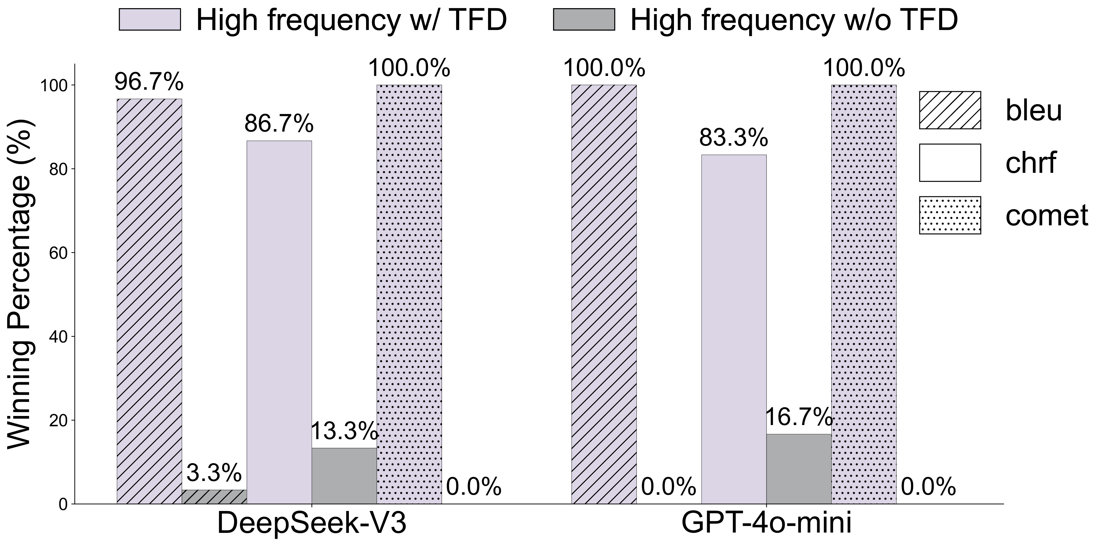
Figure 4 解读：TFD ablation 统计的是 “winning percentage”。DeepSeek-V3 中，High frequency w/ TFD 在 BLEU/chrF/COMET 上分别赢 96.7%、86.7%、100.0%，w/o TFD 仅为 3.3%、13.3%、0.0%；GPT-4o-mini 中，w/ TFD 分别为 100.0%、83.3%、100.0%，w/o TFD 为 0.0%、16.7%、0.0%。这说明用目标 LLM 生成语料修正频率估计确实比只用开放语料更强。

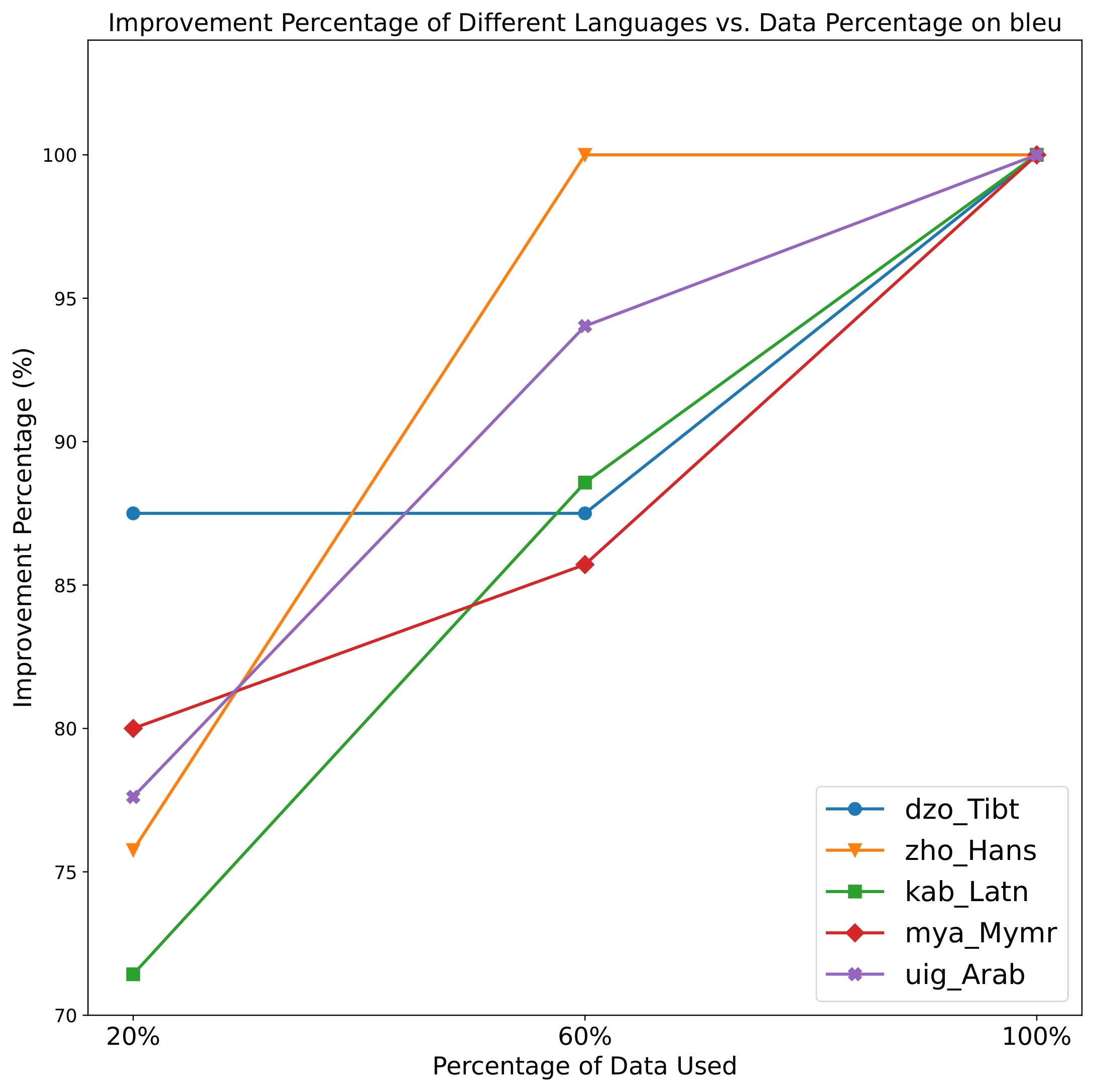
Figure 5 解读：随着 TFD 使用数据比例从 20% 到 60% 再到 100% 增加，多个语言的 BLEU improvement percentage 趋于 100%。图中 zho_Hans 在 60% 已到 100%，dzo_Tibt 在 20%/60% 约 87% 后到 100%，kab_Latn、mya_Mymr、uig_Arab 也在 100% 数据时达到 100%，说明 distilled corpus 越充分，频率估计越可靠。

复杂度分析显示，高频表达和低频表达的句法复杂度相关性很弱：MR 中 Max Dependency Tree Depth 的 Pearson/Spearman 仅 -0.0447/-0.0285，Mean Dependency Distance 为 -0.0086/0.0094，Flesch-Kincaid 为 -0.0799/-0.0545；MT 中三者分别为 -0.2713/-0.2822、-0.1137/-0.1257、-0.1673/-0.1528。因此 TFL 不是传统 easy-to-hard 的改名版。

5.5 Case study、结论与限制

Figure 6 解读：case study 展示同一语义下，高频 input 产生的 Serbian Cyrillic 翻译在 BLEU/chrF/COMET 上高于低频 input 和 original input。例如第一个 case 中，高频输出 BLEU 0.6189、chrF 51.7009、COMET 0.887192964553833；低频输出 BLEU 0.4717、chrF 36.6703、COMET 0.8209505677223206；原始输出 BLEU 0.5230、chrF 43.4805、COMET 0.8451238870620728。

整体结论是：TFL 在 prompting 和 fine-tuning 中都成立得相当稳定；TFD 能提升频率估计质量；CTFT 让高频数据优势进一步转化为 fine-tuned model 的收益。限制也很明确：TFD 需要调用 LLM 做 story completion，因此有额外计算成本；理论证明只严格支撑 frequency 与 NLL ordering，不严格证明 task performance ordering；released code 目前也缺少完整训练 launch config，并存在 CTFT 排序脚本变量未定义/方向需要核对的复现风险。

Paper Notes

探索

Adam's Law: Textual Frequency Law on Large Language Models