Kimi K2.5: Visual Agentic Intelligence

Authors: Kimi Team (325+ contributors, alphabetical order) Affiliations: Moonshot AI, The University of Hong Kong arXiv: 2602.02276 Project Page: www.kimi.com/ai-models/kimi-k2-5 GitHub: MoonshotAI/Kimi-K2.5

1. Motivation (研究动机)

当前大语言模型正在快速向 agentic intelligence 方向演进。GPT-5.2、Claude Opus 4.5、Gemini 3 Pro 等模型在 tool calling 和多步推理方面展现了强大能力，但仍存在两个核心瓶颈：

1. 文本与视觉的割裂优化：传统多模态模型通常将视觉能力作为语言模型的后期附加（post-hoc add-on），在后期引入大比例视觉 token。这种方式导致两种模态之间无法充分协同增强，视觉推理和文本推理存在能力断层。

2. 单 agent 顺序执行的延迟瓶颈：现有 agentic 系统依赖顺序的 tool calling 和推理步骤，推理时间随任务复杂度线性增长。当任务涉及大规模研究、设计、开发等异构子问题时，单 agent 范式变得低效且不可扩展。

Kimi K2.5 针对这两个问题提出了系统性解决方案：通过 joint text-vision optimization 实现两种模态的双向增强，通过 Agent Swarm 框架实现并行 agent 编排，将任务复杂度从线性扩展转为并行处理。

2. Idea (核心思想)

Kimi K2.5 的核心创新思想可总结为三点：

1. Joint Optimization 双向增强：文本和视觉不应独立优化，而应在 pre-training、SFT、RL 三个阶段全程联合优化。关键发现是 early fusion with lower vision ratio 比 late fusion with high vision ratio 效果更好；text-only SFT（zero-vision SFT）反而能激活视觉 agentic 能力；visual RL 不仅提升视觉性能，还能通过 cross-modal transfer 提升文本推理。

2. Zero-Vision SFT 范式：后训练阶段仅用纯文本 SFT 数据，通过 IPython 编程操作代理图像处理，即可激活视觉 tool-use 能力。这避免了人工标注视觉 CoT 数据的局限性。

3. Agent Swarm 并行编排：不再将复杂任务作为推理链顺序执行，而是由可训练的 orchestrator 动态分解任务、创建领域专用 subagent、并行调度执行。通过 Parallel-Agent Reinforcement Learning (PARL) 训练 orchestrator 学习何时、如何并行化。

3. Method (方法)

3.1 总体框架

Kimi K2.5 基于 Kimi K2 构建，是一个 1.04 万亿参数的 Mixture-of-Experts (MoE) transformer 模型，每个 token 激活 32B 参数（384 experts，sparsity 8/48）。训练流程包含：ViT Training → Joint Pre-training → Long-context Mid-training → SFT → Joint RL。

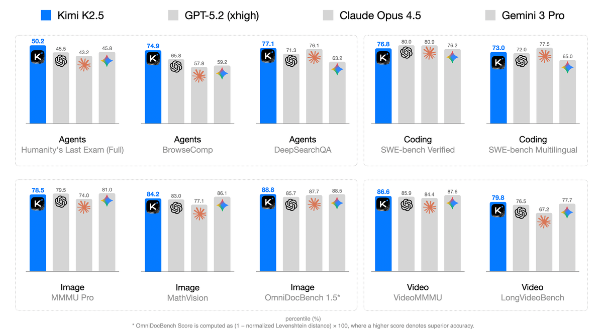
Figure 1 解读：Kimi K2.5 在 Agent、Coding、Image、Video 四大类共 10 个 benchmark 上与 GPT-5.2、Claude Opus 4.5、Gemini 3 Pro 的对比（percentile 排名）。K2.5 在 Agents 类别（HLE Full、BrowseComp、DeepSearchQA）和 Video 类别（LongVideoBench）上取得最优或接近最优表现，在 Coding（SWE-bench Verified/Multilingual）和 Image（MMMU Pro、MathVision、OmniDocBench）上与顶级闭源模型竞争力相当。

3.2 模型架构 - MoonViT-3D

多模态架构包含三个组件：

• MoonViT-3D：三维原生分辨率视觉编码器，基于 SigLIP-SO-400M 初始化，采用 NaViT packing strategy 支持变分辨率输入
• MLP Projector：连接视觉编码器和语言模型
• Kimi K2 MoE LLM：1.04T 参数的 MoE 语言模型

MoonViT-3D 的核心设计是将 “patch n’ pack” 理念推广到时间维度：将最多 4 个连续视频帧作为 spatiotemporal volume 处理，2D patches 联合展平并打包为单一 1D 序列。这实现了：

• 图像和视频共享同一参数空间和特征表示
• 无需专门的视频模块或架构分叉
• 通过 temporal pooling 实现 $4\times$ 时间压缩，显著延长可处理的视频长度

# MoonViT-3D: 3D Vision Transformer with temporal compression
class MoonViT3D:
    def __init__(self, base_model="SigLIP-SO-400M"):
        self.vit = load_pretrained(base_model)  # NaViT packing strategy
        self.temporal_pool = TemporalPooling(factor=4)
 
    def encode(self, visual_input):
        """Process images or videos with shared parameters."""
        if visual_input.is_video:
            # Group consecutive frames into chunks of 4
            chunks = group_frames(visual_input, chunk_size=4)
            all_patches = []
            for chunk in chunks:
                # Treat 4 frames as spatiotemporal volume
                # Flatten 2D patches from all frames into 1D sequence
                patches = self.vit.patchify_3d(chunk)  # [N_patches, D]
                all_patches.append(patches)
            features = self.vit.forward(concat(all_patches))
            # Lightweight temporal pooling: 4x compression
            features = self.temporal_pool(features)
        else:
            # Native resolution image processing
            patches = self.vit.patchify(visual_input)
            features = self.vit.forward(patches)
        return features

3.3 Native Multimodal Pre-Training

Figure 9 解读：不同 vision-text 联合训练策略的对比。传统方法在训练后期引入高比例视觉 token（Late fusion, 50%:50%），而 Kimi K2.5 采用 early fusion with low vision ratio（10%:90%），在固定的 vision-text token 预算下取得更优的多模态性能。

关键发现：在总 vision-text token 预算固定的前提下，early fusion with lower vision ratio 效果更好。

Vision Injection Timing	Vision-Text Ratio	Vision Knowledge	Vision Reasoning	OCR	Text Knowledge	Text Reasoning	Code
Early (0%)	10%:90%	25.8	43.8	65.7	45.5	58.5	24.8
Mid (50%)	20%:80%	25.0	40.7	64.1	43.9	58.6	24.0
Late (80%)	50%:50%	24.2	39.0	61.5	43.1	57.8	24.0

Pre-training 共三个阶段，处理约 15T tokens：

阶段	ViT Training	Joint Pre-training	Long-context Mid-training
数据	Alt text, Synthesis Caption, Grounding, OCR, Video	+ Text, Knowledge, Interleaving, Video, OS Screenshot	+ High-quality Text & Multimodal, Long Video, Reasoning, Long-CoT
序列长度	4096	4096	32768 → 262144
Tokens	1T	15T	500B → 200B
训练模块	ViT	ViT & LLM	ViT & LLM

# Pre-training pipeline for Kimi K2.5
class KimiK25PreTraining:
    def __init__(self):
        self.vit = MoonViT3D()          # Stage 1: ViT-only training
        self.projector = MLPProjector()
        self.llm = KimiK2MoE()          # 1.04T params, 32B activated
 
    def stage1_vit_training(self, data):
        """ViT training on image-text and video-text pairs.
        Uses cross-entropy caption loss (no contrastive loss).
        Two sub-stages: (1) align ViT with Moonlight-16B-A3B,
        (2) update only MLP projector to bridge ViT with 1T LLM."""
        for batch in data:  # ~1T tokens, seq_len=4096
            visual_features = self.vit.encode(batch.images)
            projected = self.projector(visual_features)
            loss = cross_entropy_caption_loss(
                self.llm(projected, batch.text), batch.targets
            )
            loss.backward()  # Only update ViT parameters
 
    def stage2_joint_pretraining(self, data):
        """Joint pre-training with early vision fusion at 10%:90% ratio.
        Introduces unique tokens, increased coding weight."""
        for batch in data:  # ~15T tokens, seq_len=4096
            loss = self.forward_multimodal(batch)
            loss.backward()  # Update ViT & LLM jointly
 
    def stage3_midtraining(self, data):
        """Long-context mid-training with YaRN interpolation.
        Extends context from 32K to 262K tokens."""
        for batch in data:  # 500B->200B tokens, seq_len=32768->262144
            loss = self.forward_multimodal(batch)
            loss.backward()  # Update ViT & LLM

3.4 Zero-Vision SFT

传统多模态 SFT 需要人工标注视觉 CoT 数据（如 crop、rotate、flip 操作），数据有限且多样性不足。Kimi K2.5 提出 zero-vision SFT：仅用纯文本 SFT 数据即可激活视觉 agentic 能力。

核心机制是将所有图像处理操作通过 IPython 编程接口代理，例如：

• 通过 binarization 和 counting 实现像素级操作
• 通过编程实现 object localization、counting、OCR

这种 “zero-vision” 激活之所以有效，是因为 joint pre-training 已经建立了强大的 vision-text alignment，文本 SFT 的能力可以自然泛化到视觉模态。

Figure 2 解读：从 zero-vision SFT 出发的 vision RL 训练曲线。四个 benchmark（MMMU Pro、MathVision、CharXiv(RQ)、OCRBench）的性能随 RL FLOPs 增加持续提升，证明 zero-vision 激活配合长期 RL 训练足以获得强大的视觉能力。

# Zero-Vision SFT: activate visual capabilities using text-only data
class ZeroVisionSFT:
    def __init__(self, model):
        self.model = model
 
    def create_training_data(self):
        """Use only text SFT data. Image manipulations are proxied
        through programmatic operations in IPython."""
        text_sft_data = load_text_sft_corpus()
        # No vision-specific SFT data needed!
        # All image operations expressed as code:
        # e.g., "Use Python to count objects in the image"
        #       "Write code to extract text via OCR"
        #       "Compute bounding boxes programmatically"
        return text_sft_data
 
    def train(self, data):
        """Standard SFT on text-only data.
        Joint pre-training ensures cross-modal generalization."""
        for batch in data:
            logits = self.model(batch.input_ids)
            loss = cross_entropy(logits, batch.targets)
            loss.backward()

3.5 Joint Multimodal Reinforcement Learning

RL 阶段包含两个关键创新：outcome-based visual RL 和 joint multimodal RL。

Outcome-Based Visual RL 针对三类任务：

• Visual grounding and counting
• Chart and document understanding
• Vision-critical STEM problems

Cross-Modal Transfer：visual RL 不仅提升视觉性能，还意外改善了文本基准：

Benchmark	Before Vision-RL	After Vision-RL	Improvement
MMLU-Pro	84.7	86.4	+1.7
GPQA-Diamond	84.3	86.4	+2.1
LongBench v2	56.7	58.9	+2.2

Joint Multimodal RL 按能力域（而非模态）组织 RL 训练：knowledge、reasoning、coding、agentic 等 domain experts 同时从纯文本和多模态查询学习，Generative Reward Model (GRM) 跨异构 traces 优化。

Figure (RL Framework) 解读：Kimi K2.5 的强化学习框架示意图，展示了 joint text-vision RL 的整体流程，包括 policy optimization、reward function、以及 GRM 的协同工作方式。

Policy Optimization 使用 token 级别的 clipping 机制：

$$L_{\text{RL}}(\theta )={\mathbb{E}}_{x\sim \mathcal{D}}\left[\frac{1}{N}\sum _{j=1}^K\sum _{i=1}^{|y_j|}\text{Clip}\left(\frac{{\pi }_{\theta }(y_j^i|x,y_j^{0:i})}{{\pi }_{\text{old}}(y_j^i|x,y_j^{0:i})},\alpha ,\beta \right)(r(x,y_j)-\bar{r}(x))-\tau {\left(\log \frac{{\pi }_{\theta }(y_j^i|x,y_j^{0:i})}{{\pi }_{\text{old}}(y_j^i|x,y_j^{0:i})}\right)}^2\right]$$

其中 $\alpha ,\beta ,\tau >0$ 为超参数，$y_{0:i}^j$ 是第 $j$ 个 response 中前 $i$ 个 token 的前缀，$N={\sum }_{j=1}^K|y_j|$ 是 batch 中生成 token 的总数，$\bar{r}(x)=\frac{1}{K}{\sum }_{j=1}^{K}r(x,y_j)$ 是所有生成 response 的 reward 均值。

关键区别于标准 PPO clipping：本方法严格依赖 log-ratio 本身（而非 advantage 的符号）来 bound off-policy drift，log-ratio 在 $[\alpha ,\beta ]$ 范围内正常计算梯度，超出范围则梯度归零。

Reward Function 设计：

• Rule-based outcome reward：用于可验证任务（数学、编程等）
• Budget-control reward：优化 token 效率
• GRM（Generative Reward Models）：用于开放式任务的细粒度评估
• 视觉特定 reward：grounding 用 F1-based soft matching（IoU），point localization 用 Gaussian-weighted distance，polygon segmentation 用 rasterize + IoU，OCR 用 normalized edit distance，counting 用 absolute difference

# Joint Multimodal RL with token-level clipping
class JointMultimodalRL:
    def __init__(self, model, reward_fn, grm):
        self.policy = model
        self.old_policy = deepcopy(model)
        self.reward_fn = reward_fn
        self.grm = grm
        self.optimizer = MuonClipOptimizer()
 
    def compute_loss(self, x, responses, alpha, beta, tau):
        """Token-level clipped policy optimization."""
        rewards = [self.reward_fn(x, y) for y in responses]
        mean_reward = mean(rewards)
        total_loss = 0
        N = sum(len(y) for y in responses)
 
        for j, y in enumerate(responses):
            advantage = rewards[j] - mean_reward
            for i in range(len(y)):
                prefix = y[:i]
                log_ratio = (
                    self.policy.log_prob(y[i], x, prefix)
                    - self.old_policy.log_prob(y[i], x, prefix)
                )
                # Clip: gradients zeroed if log_ratio outside [alpha, beta]
                ratio = clip(exp(log_ratio), alpha, beta)
                policy_loss = ratio * advantage
                kl_penalty = tau * log_ratio ** 2
                total_loss += (policy_loss - kl_penalty) / N
        return -total_loss
 
    def compute_visual_reward(self, task_type, prediction, ground_truth):
        """Task-specific visual rewards."""
        if task_type == "grounding":
            return f1_soft_match_iou(prediction, ground_truth)
        elif task_type == "point_localization":
            return gaussian_weighted_distance(prediction, ground_truth)
        elif task_type == "polygon_segmentation":
            mask = rasterize_polygon(prediction)
            return compute_iou(mask, ground_truth)
        elif task_type == "ocr":
            return 1.0 - normalized_edit_distance(prediction, ground_truth)
        elif task_type == "counting":
            return 1.0 - abs(prediction - ground_truth) / max(ground_truth, 1)

3.6 Token Efficient RL - Toggle

Toggle 是一种交替训练启发式方法，在 inference-time scaling 和 budget-constrained optimization 之间切换：

$$\tilde{r}(x,y)=\{\begin{array}{ll}r(x,y)\cdot \mathbb{I}\left\{\frac{1}{K}{\sum }_{i=1}^{K}r(x,y_i)<\lambda \text{ or }|y_i|\le \text{budget}(x)\right\}& \text{if }\lfloor t/m\rfloor (\mathrm{mod}2)=0\text{ (Phase0)}\\ r(x,y)& \text{if }\lfloor t/m\rfloor (\mathrm{mod}2)=1\text{ (Phase1)}\end{array}$$

其中 budget 由正确 response 长度的 $\rho$-th percentile 估计：

$$\text{budget}(x)=\text{Percentile}\left(\{|y_j|\mid r(x,y_i)=1,i=1,\dots ,K\},\rho \right)$$

• Phase 0 (budget limited)：在任务相关的 token budget 内求解，仅当模型平均 accuracy 超过阈值 $\lambda$ 时强制执行
• Phase 1 (standard scaling)：生成到最大 token 限制，鼓励 inference-time scaling

Toggle 平均减少输出 token 25~30%，性能几乎无损。

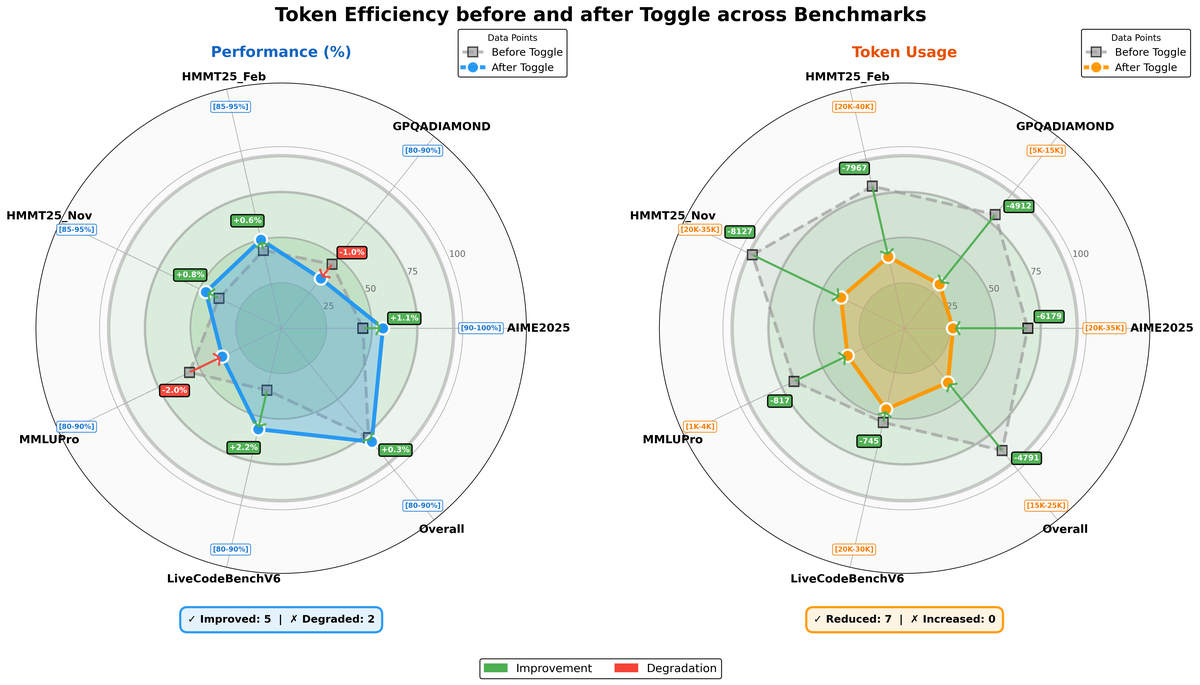
Figure 5 解读：Toggle 前后在多个 benchmark 上的性能和 token 使用量对比（雷达图）。左图显示性能基本维持（5 improved, 2 degraded），右图显示 token 使用量在所有 benchmark 上均有明显减少（7 reduced, 0 increased），证明 Toggle 有效提升了 token 效率。

# Toggle: alternating inference-time scaling and budget-constrained RL
class ToggleRL:
    def __init__(self, lambda_threshold, rho_percentile, m_period):
        self.lambda_t = lambda_threshold  # accuracy threshold
        self.rho = rho_percentile         # budget percentile
        self.m = m_period                 # alternation period
 
    def estimate_budget(self, x, responses, rewards):
        """Estimate problem-dependent token budget from correct responses."""
        correct_lengths = [
            len(y) for y, r in zip(responses, rewards) if r == 1
        ]
        if not correct_lengths:
            return float('inf')
        return percentile(correct_lengths, self.rho)
 
    def compute_reward(self, x, y, t, K, all_responses, all_rewards):
        """Toggle reward: alternate between budget-limited and scaling."""
        r = base_reward(x, y)
        phase = (t // self.m) % 2
 
        if phase == 0:  # Budget limited phase
            mean_acc = mean(all_rewards)
            budget = self.estimate_budget(x, all_responses, all_rewards)
            if mean_acc < self.lambda_t or len(y) <= budget:
                return r
            else:
                return 0  # Penalize exceeding budget when accuracy is high
        else:  # Standard scaling phase
            return r

3.7 Agent Swarm 与 PARL

Figure 3 解读：Agent Swarm 架构图。一个可训练的 Orchestrator 动态创建领域专用 subagent（AI Researcher、Physics Researcher、Life Sciences Researcher、Fact Checker、Web Developer 等），将复杂任务分解为可并行执行的子任务。Orchestrator 拥有 create_subagent、assign_task、search、browser 等工具。子任务结果汇聚回 Orchestrator 进行最终整合。

架构设计：

• Orchestrator：可训练的，负责任务分解、subagent 创建和调度
• Subagents：冻结的，从固定的中间策略 checkpoint 实例化，执行具体子任务
• 训练时仅更新 orchestrator，subagent 的输出被视为环境观测（environmental observations）

PARL Reward 定义为三项之和：

$$r_{\text{PARL}}(x,y)={\lambda }_1\cdot \underset{\text{instantiation reward}}{\underbrace{r_{\text{parallel}}}}+{\lambda }_2\cdot \underset{\text{sub-agent finish rate}}{\underbrace{r_{\text{finish}}}}+\underset{\text{task-level outcome}}{\underbrace{r_{\text{perf}}(x,y)}}$$

• $r_{\text{parallel}}$：鼓励并行 subagent instantiation，防止 serial collapse（退化为单 agent 顺序执行）
• $r_{\text{finish}}$：防止 spurious parallelism（大量 spawn subagent 但无实际完成）
• $r_{\text{perf}}$：任务级最终性能 reward
• ${\lambda }_1,{\lambda }_2$ 在训练过程中退火到零，确保最终策略优化主目标

Critical Steps 指标：

$$\text{CriticalSteps}=\sum _{t=1}^T\left(S_{\text{main}}^{(t)}+\underset{i}{\max }{S}_{\text{sub},i}^{(t)}\right)$$

其中 $T$ 为执行阶段数，$S_{\text{main}}^{(t)}$ 为第 $t$ 阶段主 agent 步数（通常为 1），$S_{\text{sub},i}^{(t)}$ 为第 $i$ 个 subagent 的步数。该指标衡量关键路径长度（wall-clock time），鼓励均衡的任务分解以缩短最长并行分支。

Figure 4 解读：PARL 训练过程中 training accuracy（左）和 average parallelism（右）随 RL FLOPs 的变化。两个指标同步平滑增长，说明 orchestrator 通过 RL 逐步学会更有效的并行任务分解策略。

# Agent Swarm with Parallel-Agent Reinforcement Learning (PARL)
class AgentSwarm:
    def __init__(self, orchestrator, subagent_checkpoint):
        self.orchestrator = orchestrator        # Trainable
        self.subagent_policy = subagent_checkpoint  # Frozen
 
    def execute(self, task):
        """Orchestrator decomposes task and manages parallel subagents."""
        # Step 1: Orchestrator analyzes task and creates subagents
        plan = self.orchestrator.plan(task)
        subagents = []
        for spec in plan.subagent_specs:
            agent = self.create_subagent(spec.role, spec.tools)
            subagents.append(agent)
 
        # Step 2: Assign tasks to subagents (parallel execution)
        futures = []
        for agent, subtask in zip(subagents, plan.subtasks):
            future = parallel_execute(agent, subtask)  # Non-blocking
            futures.append(future)
 
        # Step 3: Collect results and synthesize final answer
        results = [f.result() for f in futures]
        return self.orchestrator.synthesize(task, results)
 
    def create_subagent(self, role, tools):
        """Dynamically instantiate domain-specific frozen subagent."""
        return SubAgent(
            policy=self.subagent_policy,  # Fixed checkpoint
            role=role,       # e.g., "AI Researcher", "Fact Checker"
            tools=tools      # e.g., [search, browser, code_exec]
        )
 
 
class PARLTrainer:
    def __init__(self, lambda1, lambda2):
        self.lambda1 = lambda1  # Annealed to 0 during training
        self.lambda2 = lambda2  # Annealed to 0 during training
 
    def compute_parl_reward(self, x, y, subagent_results):
        """PARL reward = instantiation + finish rate + performance."""
        r_parallel = self.parallel_instantiation_reward(y)
        r_finish = self.subagent_finish_rate(subagent_results)
        r_perf = self.task_performance_reward(x, y)
        return self.lambda1 * r_parallel + self.lambda2 * r_finish + r_perf
 
    def compute_critical_steps(self, episode):
        """Measure wall-clock proxy: critical path length."""
        total = 0
        for stage in episode.stages:
            main_steps = stage.main_agent_steps  # typically 1
            max_sub_steps = max(
                (sub.steps for sub in stage.subagents), default=0
            )
            total += main_steps + max_sub_steps
        return total

3.8 Decoupled Encoder Process (DEP)

针对多模态训练中 Pipeline Parallelism 的 load imbalance 问题，提出 Decoupled Encoder Process (DEP)：

1. Balanced Vision Forward：先对全局 batch 中所有视觉数据执行 forward pass，在所有 GPU 上均匀分配（按 image/patch count 负载均衡），丢弃中间激活仅保留最终输出
2. Backbone Training：主 transformer backbone 执行标准的 forward/backward pass，可完全复用纯文本训练的高效并行策略
3. Vision Recomputation & Backward：重计算视觉 encoder forward pass，然后执行 backward pass 计算视觉参数梯度

DEP 实现了多模态训练效率达到纯文本训练的 90%。

# Decoupled Encoder Process (DEP) for efficient multimodal training
class DecoupledEncoderProcess:
    def __init__(self, vit, llm, num_pp_stages):
        self.vit = vit
        self.llm = llm
 
    def training_step(self, batch):
        # Phase 1: Balanced Vision Forward (all GPUs)
        # Distribute visual data evenly across all GPUs by load metrics
        visual_data = distribute_by_load(batch.visual, metric="patch_count")
        with no_grad():  # Discard intermediate activations
            vit_outputs = self.vit(visual_data)
        # Gather outputs back to PP Stage-0
        vit_features = all_gather_to_stage0(vit_outputs)
 
        # Phase 2: Backbone Training (standard PP strategy)
        # Forward + backward for main transformer
        llm_output = self.llm.forward(batch.text, vit_features)
        llm_output.backward()  # Gradients accumulated at ViT output
 
        # Phase 3: Vision Recomputation & Backward
        # Recompute ViT forward (needed for gradients)
        vit_outputs_recomputed = self.vit(visual_data)
        vit_outputs_recomputed.backward(grad_from_llm)

3.9 代码到论文映射表

Paper Concept	Source File	Key Class/Function
模型权重	HuggingFace: moonshotai/Kimi-K2.5	模型 checkpoint
部署指南	docs/deploy_guidance.md	部署配置
技术报告 PDF	tech_report.pdf	完整技术报告

注：GitHub 仓库仅包含模型权重发布和部署指南，未公开训练代码。上述 pseudocode 基于论文描述编写。

4. Experimental Setup (实验设置)

Benchmarks 分类

• Reasoning & General: HLE, AIME 2025, HMMT 2025 (Feb), IMO-AnswerBench, GPQA-Diamond, MMLU-Pro, SimpleQA Verified, AdvancedIF, LongBench v2
• Coding: SWE-Bench Verified, SWE-Bench Pro (public), SWE-Bench Multilingual, Terminal Bench 2.0, PaperBench (CodeDev), CyberGym, SciCode, OJBench (cpp), LiveCodeBench (v6)
• Agentic: BrowseComp, WideSearch, DeepSearchQA, FinSearchCompT2&T3, Seal-0, GDPVal
• Image Understanding: MMMU-Pro, MMMU (val), CharXiv (RQ), MathVision, MathVista (mini), SimpleVQA, WorldVQA, ZeroBench, BabyVision, BLINK, MMVP, OmniDocBench 1.5, OCRBench, InfoVQA (test)
• Video Understanding: VideoMMU, MMVU, MotionBench, Video-MME (with subtitles), LongVideoBench, LVBench
• Computer Use: OSWorld-Verified, WebArena

Baselines

• 闭源模型: Claude Opus 4.5 (extended thinking), GPT-5.2 (xhigh reasoning effort), Gemini 3 Pro (high reasoning-level)
• 开源模型: DeepSeek-V3.2 (thinking mode enabled), Qwen3-VL-235B-A22B-Thinking

评估配置

• Temperature = 1.0, top-p = 0.95
• Context length = 256k tokens
• 无公开分数的 benchmark 使用相同条件重新评估（标记 *）

5. Experimental Results (实验结果)

5.1 主要结果（Table 4 精选）

Benchmark	Kimi K2.5	Claude Opus 4.5	GPT-5.2	Gemini 3 Pro
Reasoning
HLE-Full	30.1	30.8	34.5	37.5
HLE-Full w/ tools	50.2	43.2	45.5	45.8
AIME 2025	96.1	92.8	100	95.0
HMMT 2025 (Feb)	95.4	92.9*	99.4	97.3*
GPQA-Diamond	87.6	87.0	92.4	91.9
MMLU-Pro	87.1	89.3*	86.7*	90.1
Coding
SWE-Bench Verified	76.8	80.9	80.0	76.2
SWE-Bench Multilingual	73.0	77.5	72.0	65.0
LiveCodeBench (v6)	85.0	82.2*	-	87.4*
Agentic
BrowseComp	60.6	37.0	65.8	37.8
BrowseComp (Agent Swarm)	78.4	-	-	-
WideSearch	72.7	-	76.2*	57.0
WideSearch (Agent Swarm)	79.0	-	-	-
DeepSearchQA	77.1	76.1*	71.3*	63.2*
Image
MMMU-Pro	78.5	74.0	79.5*	81.0
MathVision	84.2	77.1*	83.0	86.1*
OmniDocBench 1.5	88.8	87.7*	85.7	88.5
OCRBench	92.3	86.5*	80.7*	90.3*
Video
VideoMMU	86.6	84.4*	85.9	87.6
LongVideoBench	79.8	67.2*	76.5*	77.7*
MotionBench	70.4	60.3*	64.8*	70.3
Computer Use
OSWorld-Verified	63.3	66.3	8.6*	20.7*
WebArena	58.9	63.4*	-	-

5.2 Token Efficiency（Table 5）

Kimi K2.5 在保持竞争力性能的同时显著降低 token 消耗：

Benchmark	Kimi K2.5 (tokens)	Kimi K2 Thinking	Gemini-3.0 Pro	DeepSeek-V3.2 Thinking
AIME 2025	96.1 (25k)	94.5 (30k)	95.0 (15k)	93.1 (16k)
HMMT Feb 2025	95.4 (27k)	89.4 (35k)	97.3 (16k)	92.5 (19k)
LiveCodeBench	85.0 (18k)	82.6 (25k)	87.4 (13k)	83.3 (16k)
GPQA Diamond	87.6 (14k)	84.5 (13k)	91.9 (8k)	82.4 (7k)

5.3 Agent Swarm Results（Table 6）

Figure 8 解读：Agent Swarm vs. Single Agent 在 WideSearch 上的执行时间对比。横轴为目标 Item-F1（30%70%），纵轴为执行时间倍数。Single Agent（红点）时间随复杂度线性增长（1.8x → 7.0x），而 Agent Swarm（蓝点）保持近常数低延迟（0.6x1.6x），实现 3x~4.5x 加速。

Benchmark	K2.5 Agent Swarm	Kimi K2.5	Claude Opus 4.5	GPT-5.2	GPT-5.2 Pro
BrowseComp	78.4	60.6	37.0	65.8	77.9
WideSearch	79.0	72.7	76.2	-	-
In-house Swarm Bench	58.3	41.6	45.8	-	-

关键结论：

• Agent Swarm 在 BrowseComp 上比单 agent 提升 17.8%（60.6% → 78.4%），超越 GPT-5.2 Pro（77.9%）
• WideSearch 上 Item-F1 从 72.7% 提升到 79.0%，超越 Claude Opus 4.5（76.2%）
• 执行延迟降低 3x~4.5x
• Agent Swarm 同时起到 proactive context management 的作用，优于 Discard-all context management

Figure 7 解读：在 BrowseComp 上，Agent Swarm（蓝线）与 Discard-all Context Management（橙线）的性能随步数的对比。Agent Swarm 通过主动的上下文分片（context sharding）始终优于被动的上下文截断策略，在更少的 critical steps 下达到更高准确率。